Quick Start
This guide takes you through your first LAVA Unstructured simulation in a few minutes: the Taylor–Green vortex, a canonical transition-to-turbulence case in a periodic box. It needs no geometry and consists of the two steps of every unstructured case — generate a mesh with the LAVA Voronoi mesher, then run the solver on it — each driven by a single small input file. The initial condition is built into the solver.
Prerequisites
Before starting, ensure you have:
- The LAVA solver and utilities installed and your environment properly set up, see the LAVA Installation Guide. You need a 3D unstructured executable (any
lavaunst.3D.NS1build). - The LAVA Voronoi mesher installed, see the Voronoi Installation Guide.
- Python with matplotlib for the
plotHist.pyutility, and optionally ParaView for the volume and iso-surface files.
The Case
The Taylor–Green vortex starts from a smooth, analytic vortical velocity field in a triply periodic box. The large initial vortices stretch, break down into ever smaller scales, and finally decay — making it the standard test of how much numerical dissipation a scheme adds to an under-resolved turbulent flow. In a box \(\mathbf{x} \in [0,1]^3\) with \(f = 2\pi\), the built-in initial condition is
with the corresponding pressure field
We run the classic configuration of Carton de Wiart et al. (2014): Reynolds number 1600, Mach number 0.1, on a uniform mesh of \(64^3\) cubic cells — a deliberately coarse resolution where the quality of the numerical scheme is visible. This is the same setup as the Cartesian Quick Start, so the two solvers can be compared directly on identical grids.
Reference: Carton de Wiart, C., Hillewaert, K., Duponcheel, M., & Winckelmans, G. (2014), "Assessment of a discontinuous Galerkin method for the simulation of vortical flows at high Reynolds number," International Journal for Numerical Methods in Fluids, 74(7), 469–493.
Note
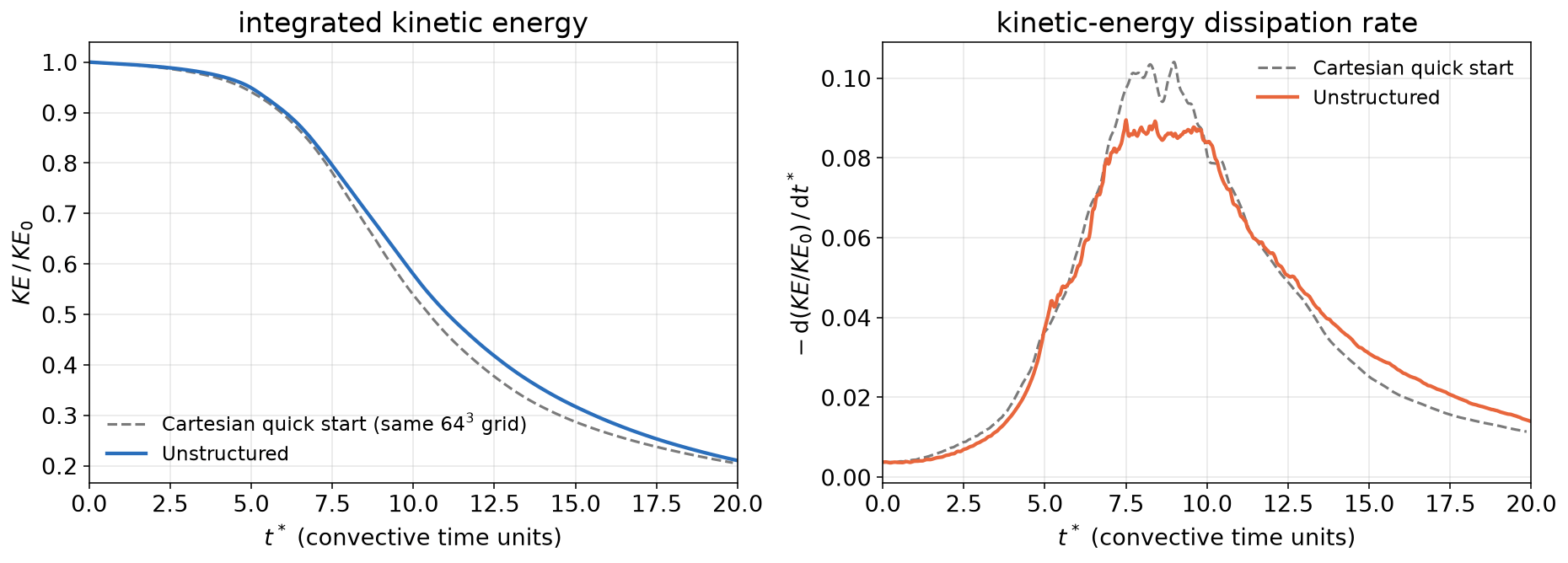
This quick start is about getting a first simulation running, not about producing a reference-quality solution: the \(64^3\) grid deliberately under-resolves the flow. Expect the results to be qualitatively right and quantitatively close — in this run the dissipation peak arrives about one and a half time units early and some 10% low compared with the reference DNS, the expected behavior of a second-order finite-volume scheme on a grid this coarse. Grid and scheme refinement studies are what the rest of the documentation is for.
Tutorial Files
Download the three input files into a working directory:
| File | Description |
|---|---|
| tgv_box.yml | Voronoi mesher input: a periodic unit box |
| tgv.inputs | solver input file |
| tg.spec | gas/species definition (sets the viscosity, i.e. the Reynolds number) |
Meshing
The unstructured solver reads its mesh from a CGNS file. Here the LAVA Voronoi Mesher generates it from the following input:
# LAVA Voronoi mesher input for the unstructured quick start: a triply
# periodic unit box filled with 64^3 cubic cells. No geometry is needed.

# Seed spacing of the finest region (spacing_rel = 1): 64 cells across the box
reference_length: 0.015625

# Fully three-dimensional mesh
2d: false

# Periodic in x, y and z: seeds near a boundary are mirrored across the
# opposite side so the cells connect seamlessly (no boundary zones are written)
periodicDir: [true, true, true]

# The lattice fits the box exactly, so no Lloyd smoothing is needed
lloyd_iter: 0

regions:
  # The first region is always the axis-aligned box that bounds the domain.
  # A cartesian seed lattice gives cubic cells; bodycentered gives the
  # truncated octahedra typically used for meshes around geometry.
  - name: box
    type: cube
    seed: cartesian
    spacing_rel: [1, 1, 1]
    distance: [1.0, 1.0, 1.0]
    center: [0.5, 0.5, 0.5]
The only region is the axis-aligned unit cube that defines the domain; the first region of every mesher input is this bounding box. Seeds are placed on a cartesian lattice with spacing reference_length, which yields \(64^3\) cubic cells. periodicDir makes all three directions periodic: seeds near a boundary are mirrored across the opposite side, so the cells connect seamlessly and the mesh has no boundary zones at all. For meshes around geometry the bodycentered seed lattice (truncated octahedra) is the usual choice — see Refinement regions in the mesher manual.
Run the mesher in the working directory (any lavavoro executable works; adjust the name to your build):
It writes tgv_box.cgns — a single volume zone of 262,144 polyhedral cells — in a few seconds.
The Input File
The complete solver input file:
# LAVA Unstructured quick start: the Taylor-Green vortex.
# A triply periodic box meshed with the Voronoi mesher; the initial condition
# is built into the solver.
exact flow name = taylorgreenvortex

time {
  steady     = false
  finish ctu = 20    # run for 20 convective time units
  cfl        = 0.8
}

reference conditions {
  velocity    = [1.0, 0, 0]
  density     = 6.283185307179586    # 2 pi
  temperature = 71.4285714285714     # gives Mach 0.1
  length      = 0.15915494309189535  # 1 / (2 pi): one classic TGV time unit per ctu
}

fluid {
  species = tg   # calorically perfect gas with constant viscosity 1/1600 (Re = 1600)
}

unst {

  grid {
    file = tgv_box.cgns
  }

  periodic {
    do lava voro periodic = true   # the mesh was built periodic by the Voronoi mesher
    xmin = 0.0
    xmax = 1.0
    ymin = 0.0
    ymax = 1.0
    zmin = 0.0
    zmax = 1.0
  }

  explicit {
    method = ssprk33   # 3rd-order strong-stability-preserving Runge-Kutta
  }

  convective terms {
    scheme                  = keepblend   # kinetic-energy/entropy-preserving flux blended with upwind
    order                   = 2
    limiter                 = none
    flux function           = ausmpw+
    upwind blending sensors = [ducrosmod]
  }

  navier stokes {
    viscous = true
  }

  output {
    monitor {
      interval  = 10
      variables = [nt, time, ctu, dt, maxcfl, maxmach, integratedke, mups]
    }
    flow_stats {
      interval = 10
    }
    volume {   # full-volume CGNS snapshots for visualization
      interval  = 500
      variables = [q, density, mach]
    }
  }
}
Walking through it block by block:
exact flow nameselects one of the analytic initial conditions built into the solver — no restart or geometry files needed.timerequests an unsteady run for 20 convective time units with an adaptive time step atcfl = 0.8.reference conditionsset the nondimensionalization: with \(V_0 = 1\), the reference temperature gives Mach 0.1, and the referencelengthof \(1/(2\pi)\) makes one convective time unit (thectumonitor column) equal to one classic Taylor–Green time unit.fluidpoints totg.spec, a calorically perfect gas with a constant viscosity of \(1/1600\) — which is the Reynolds number definition for this nondimensionalization.- Everything else lives inside the
unstblock:gridnames the mesh file — see Grid Setup.periodictells the solver that the mesh was built periodic by the Voronoi mesher (do lava voro periodic = true) and gives the box extents — see Periodic. NoBC_Nblocks are needed, since the periodic mesh has no boundary zones.explicitpicks the explicit third-order strong-stability-preserving Runge–Kutta scheme — see Explicit Stepping.convective termsselect thekeepblendscheme, the recommended low-dissipation scheme for scale-resolving simulations: a kinetic-energy and entropy preserving flux blended with an upwind flux where theducrosmodsensor detects compressibility effects — on this coarse grid a dissipative scheme would visibly damp the vortices. See Convective Terms.navier stokesswitches the viscous terms on.outputwrites a monitor line every 10 steps (with the integrated kinetic energy fromflow_stats) and a full-volume snapshot every 500 steps for visualization — see Output and Probes.
Running the Case
From the working directory, run on a few MPI ranks with a few OpenMP threads each (any lavaunst 3D NS1 executable works; adjust the name to your build):
On 64 CPU cores (8 ranks with 8 threads each) the roughly 8000 time steps take about two minutes, at some 18 million cell updates per second (the mups monitor column); reduce finish ctu for a faster first look. While it runs, the monitor table reports the state every 10 steps:
===========================================================================================================
     Time     |     Time     |     CTU      |    Time    |   Max   |   Max   |  Integrated  |   Million   |
     step     |     (s)      | (Non-dim T)  | step size  |   CFL   |  Mach   |   Kinetic    | Updates/Sec |
 (2147483637) | (3.1831e+00) | (2.0000e+01) |    (s)     |         |         |    Energy    |    n=10     |
-----------------------------------------------------------------------------------------------------------
      nt      |     time     |     ctu      |     dt     | maxcfl  | maxmach | integratedke |    mups     |
===========================================================================================================
             0     0.0000e+00         0.0000   4.0320e-04    0.8000    0.0996     7.8540e-01        0.6338 CFL^3 FlowStats^3 inputs^2 load volume
            10     4.0320e-03         0.0253   4.0320e-04    0.8000    0.0997     7.8532e-01       18.4087 CFL^10 FlowStats
            20     8.0641e-03         0.0507   4.0321e-04    0.8000    0.0997     7.8525e-01       18.3463 CFL^10 FlowStats
            30     1.2096e-02         0.0760   4.0321e-04    0.8000    0.0998     7.8517e-01       18.2731 CFL^10 FlowStats
            40     1.6128e-02         0.1013   4.0321e-04    0.8000    0.0998     7.8510e-01       18.1585 CFL^10 FlowStats
            50     2.0160e-02         0.1267   4.0321e-04    0.8000    0.0997     7.8502e-01       18.1591 CFL^10 FlowStats
Running on a GPU
LAVA Unstructured also runs on NVIDIA GPUs. Use a GPU build with one MPI rank per GPU; the input file is unchanged:
In this example the single-GPU run sustained about 60 million cell updates per second (the mups monitor column) — more than three times the throughput of the 64-core CPU run — and finished in under two minutes including the volume output; the gap grows with grid size.
Checking the Run
The monitor history is stored in monitor/Unst.data.iter. Any column can be plotted with the plotHist.py utility, e.g. the kinetic-energy decay and the maximum Mach number over convective time:
The figure below shows the integrated kinetic energy of this run and its decay rate \(-\mathrm{d}KE/\mathrm{d}t\), with the Cartesian Quick Start result on the identical \(64^3\) grid for comparison — the classic Taylor–Green result: the energy is nearly conserved while the vortices merely deform, then transition sets in and the dissipation peaks between \(t^* \approx 7\) and \(9\):
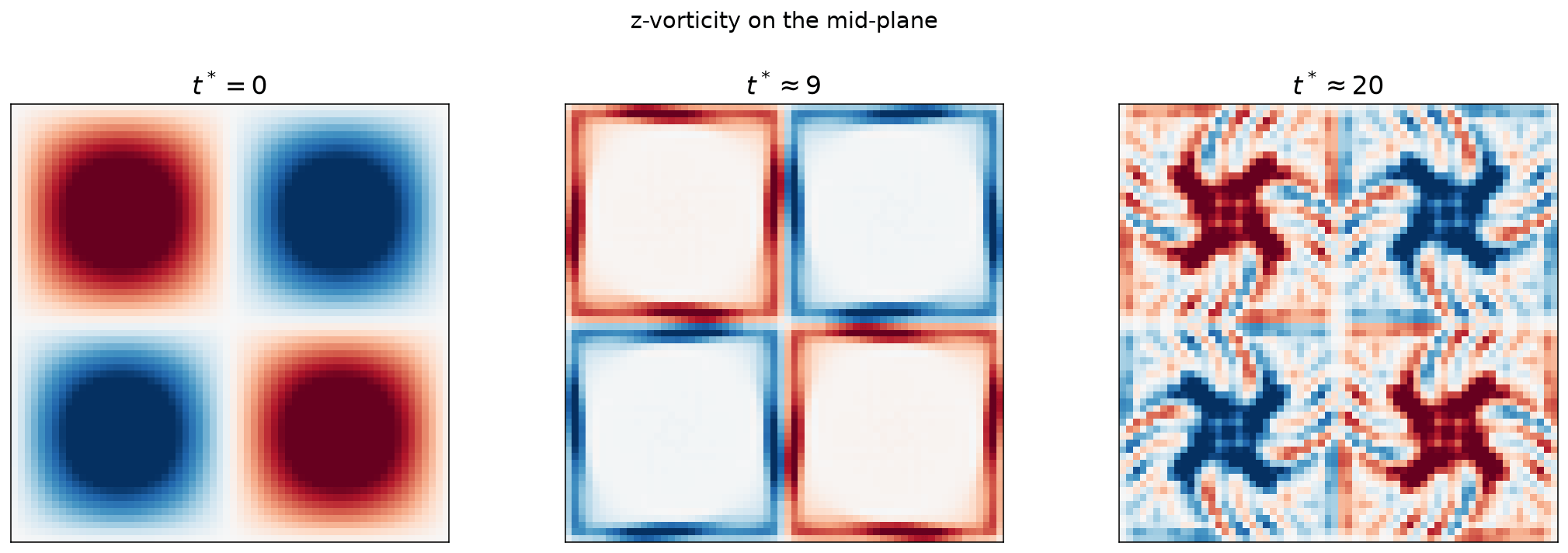
The volume snapshots land in volume/ as CGNS files (Unst.vol.*.cgns, each linking to the mesh in Unst.vol.meshLink.<step>.cgns). Open them in ParaView — remember to enable the solution arrays in the CGNS reader's Cell Arrays list. The z-vorticity on the mid-plane (a Slice through the volume) shows the smooth initial vortex array breaking down into small-scale turbulence:
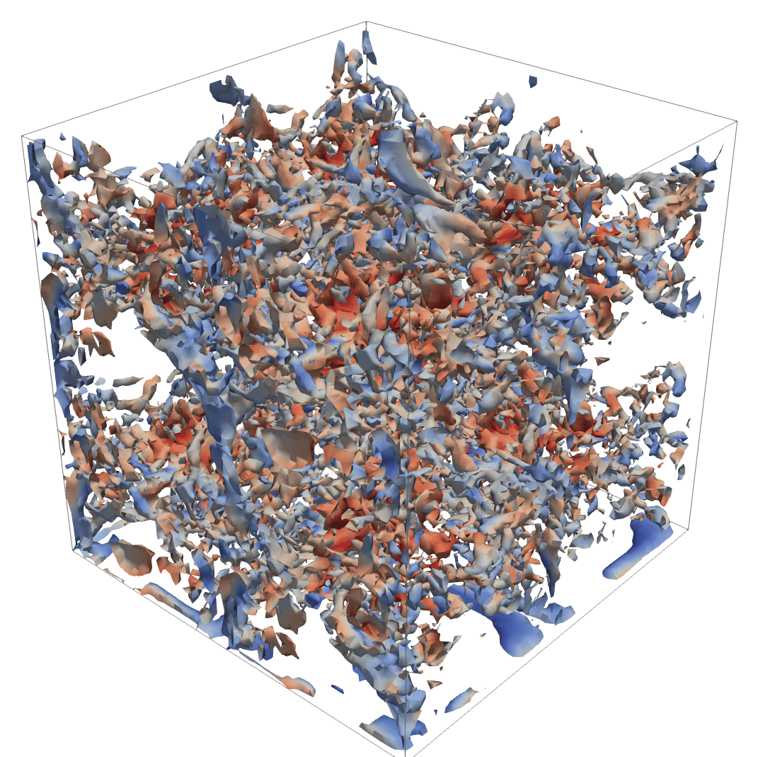
A Q-criterion iso-surface (ParaView's Gradient filter on the velocity, then Contour) shows the vortex structure. Near the dissipation peak, at \(t^* \approx 9\), the smooth initial vortices have rolled up into a dense tangle of worm vortices:
You now have a running LAVA Unstructured setup. From here:
- the mesher for real geometry: Voronoi Mesh Generator
- the full input reference: General Setup, Grid Setup, Time Integration and Numerical Schemes, Boundary Conditions, Output and Probes
- cases with geometry: the Diamond Airfoil tutorial