Project Grid Scripting
Overset gridding can be a powerful design tool because it is easy to leverage component-based buildup by gridding said components individually, altering a base set of grids efficiently, and tailor grids minutely to the requirements of problem numerics. While automated methods such as EPOGS exist, it is often still required to partially or fully script curvilinear overset grid generation for specific method requirements or grid sensitivities.
The LAVA best practices for setting up a project's grid scripting file system will be described in this tutorial. The CAD and surface grid choices made will be discussed, and the scripts to generate the volume grids overviewed. CGT is used for scripted grid generation. In the next tutorial, we will also be using an automated POGS approach to generate the volume grids for comparison, as they are sufficient for RANS analysis.
The final result of constructing a grid with a scripted project is the grid and bc files needed for subsequent tutorials. If you cannot or do not want to run this tutorial yourself, they can be downloaded here:
- grid.x: The combined CRM nearBody and octree-generated farField volume grid without iblanks.
- grid.sur: The CRM nearBody surface grids relevant to integrated loads.
- grid.bc: The combined CRM nearBody and octree-generated farField BCs.
LAVA Curvilinear Overset Project Grid Script File System
Before actually going through the process of CAD manipulation and grid generation we will discuss the scripting framework and process in which we are working. An abstract representation of a scripted project can be seen below with rough steps.
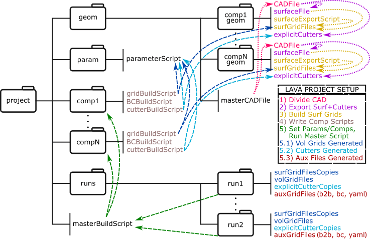
A Project requires three starting files:
- A parameter file located in a parm directory which contains information that controls how the other grid-related scripts function. Values relating to min/max allowed grid spacings, first-cell height, AOA, grid movement parameters, refinement level, etc., are held here and referenced by other files.
- A master CAD geometry located in a geom directory. This will be divided into different 'floating' component CAD files according to user preference which will be held in their own sub-directories.
- A master build script which sets which components will be built for a grid system. This script will be called in a 'run' sub directory and will sequentially look at the grid-building scripts of the relevant components.
In addition, each component will have its own directory in which its grid scripts are held, which copy and manipulate on-CAD surface grids built and held in the component's sub-directory.
The process of constructing a scripted project is usually performed in the following steps:
- Break the master CAD file into components. Usually the master CAD undergoes some cleanup first to fill gaps or remove other issues. When sectioning off a component, things to consider are how much CAD on another touching component to include for blending grids, and if gaps should be filled to create a closed geometry if cutter triangulations need to be made. Additionally, depending on your grid generation method cutting the CAD along the lines you wish your grid to follow may be beneficial.
- Export from CAD to get surface geometry (usually igs or step format) on which to build surface grids. If you want to define manual cutter triangulations from the CAD you should also export those, though often you will not realize you need them until you see issues during connectivity later.
- Build the surface grids on the geometry using a tool of choice, and then export them into plot3D format. Depending on your gridding method, you may export triangulations instead on which surface grids can be grown, e.g. via CGT scripting. How you choose to build/export your surfaces comes down to how you want to script their volume construction, and so is driven by personal preference. Depending on preference, you can export multiple sets of surface grids at various refinement levels here, if they can be refined on the CAD, or, as is done in this tutorial, perform refinement on the entire grid system later with an appropriate tool. Note that if you have a method or reason to manually build the volume grids (e.g. for wake grids) you can just build and export them here as well.
- Write the components' grid scripts. There are usually three scripts:
- Grid script: copies each surface grid from the component geometry sub-directory, then manipulates it and builds its volume grids. The settings of the volume construction are gleaned from the parameter file. Note that volume grids built in the geom sub-directory can just be copied in by this script, but they may still be manipulated depending on your parameter settings (pitch/yaw, etc) or tiling (e.g. the vanes of a wind tunnel).
- BC script: defines the BCs for each volume side built in the grid script. Each of the six sides can have partial BCs on them. If a portion or whole side doesn't have a BC, a block-to-block (B2B) with another volume will be attempted to be found later. If none is found, the side is assumed to be overset. Note that each volume side must either be completely covered with BCs and/or B2Bs OR be entirely overset.
- Cutter script: if manual cutters triangulations have been created in the component geometry sub-directory, they are copied in here and manipulated based on the parameter file (pitch, yaw, etc).
- Build a grid system: by making a sub-directory to run in, naming it after the desired parameters set in the parameter script and the components defined in the master build script. The master script is then run from within the run sub-directory. The grids and cutters built from the component scripts called are all built within the run sub-directory. Additionally, auxiliary data may be built such as yaml input files if scripts are set up to generate them. If this script is ever re-run and a component's scripts or volume grid exist and haven't been modified, that component won't be re-built.
Building the CRM Project NearBody Grid
To build the starting nearBody CRM project grid, you would simply make a new sub-folder in the 'run' directory (e.g. 'RANS'), then run the 'buildProjectGrid_nearBody.tcl' while in that folder (do not copy it in). However, do not do so yet: we will be building the entire grid system later including the offBody with a separate wrapping script.
While the CRM components' surface grids and scripts are provided in order to build the full grid while following this tutorial, the broken-up portions of the master CAD for each component are not (though they are visualized and discussed below). It is highly recommended that new users attempt this process from scratch to become familiar with CGT grid scripting and the thought process behind how to break up CAD and build surfaces with volume grid generation in mind. An example of this may be first attempting to re-create the surface grids provided, then trying different surface grid topologies.
Master and Component CAD
Some forethought should be put into cleaning up the master CAD file and breaking it into component CAD so that building surface grids on them is easier:
- Ensure that the CAD is properly segmented between features, cutting it if not.
- Ensure that no undesired open edges exist and that any spurious/sliver features are removed/repaired.
- Similarly, cut the CAD to ensure feature lines you want respected are explicitly known.
- It may be easier to pre-define the limits of particular surface grids by cutting out CAD surfaces in their final shape. Multiple of these CAD surfaces can overlap and be held in the same CAD component file.
- After cutting out a portion of the master CAD for a component, you may need to fill holes in that component to have a closed surface on which to grow the grid. This matter especially if you will be conducting a component build-up.
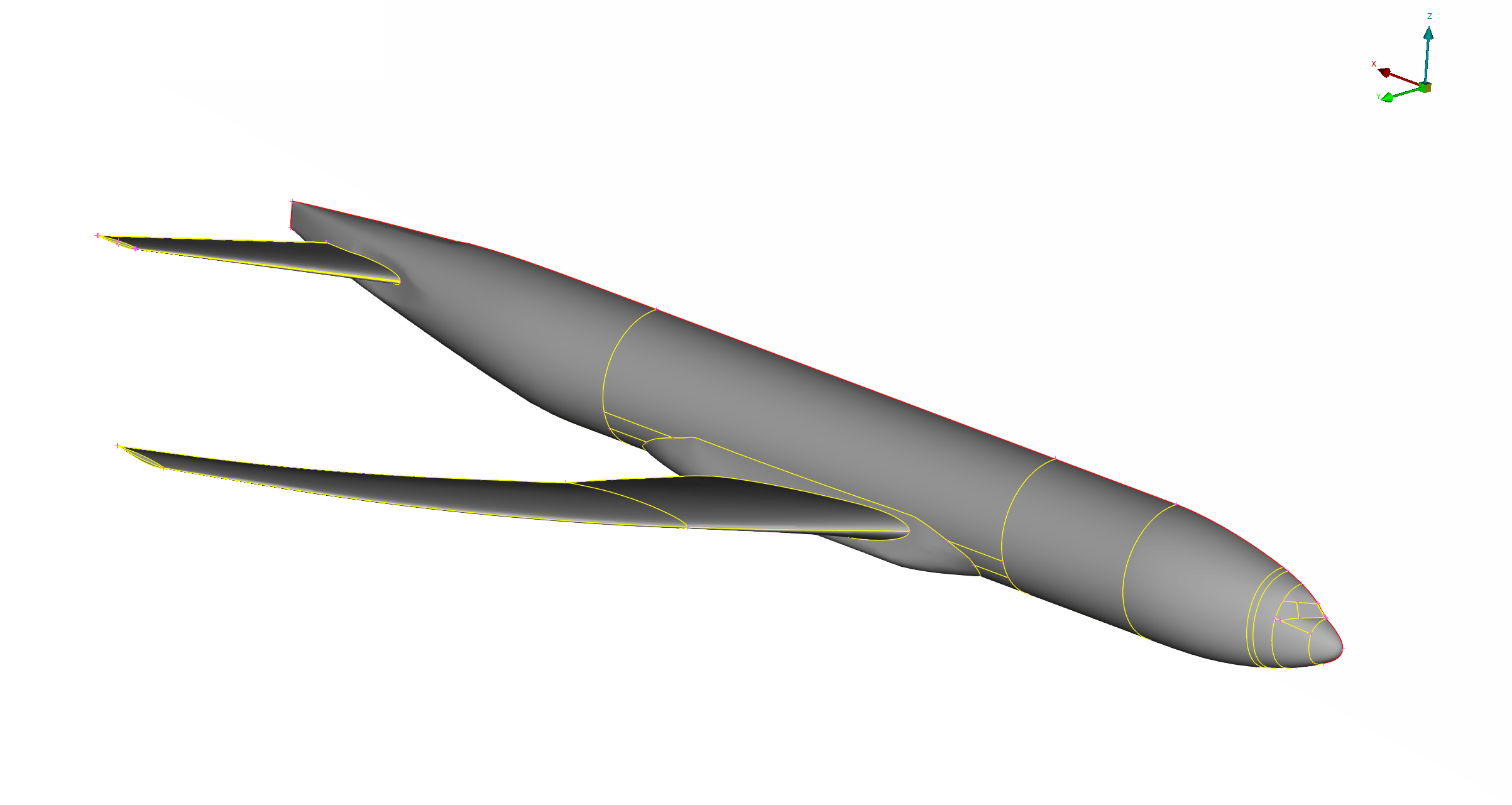
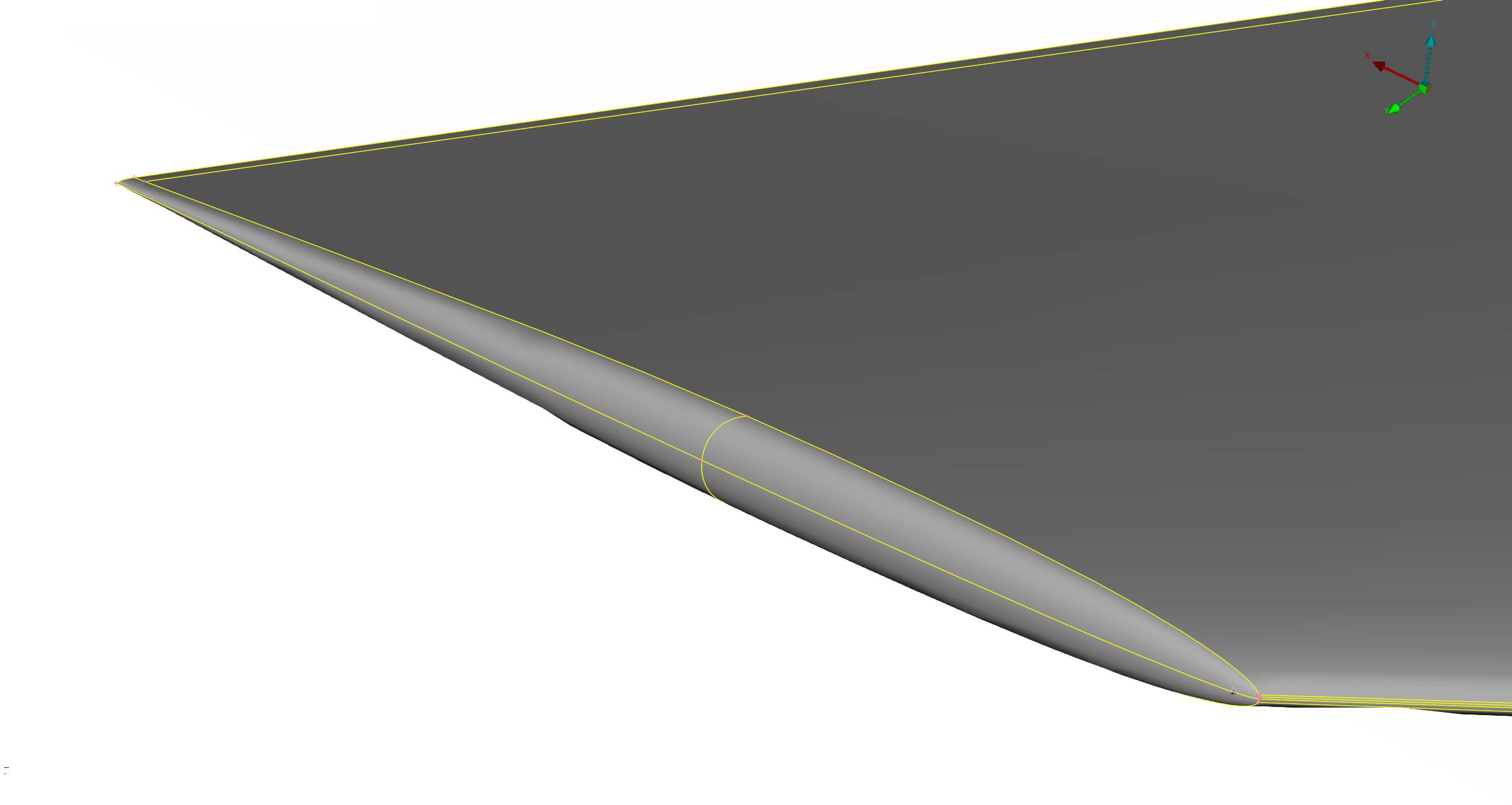
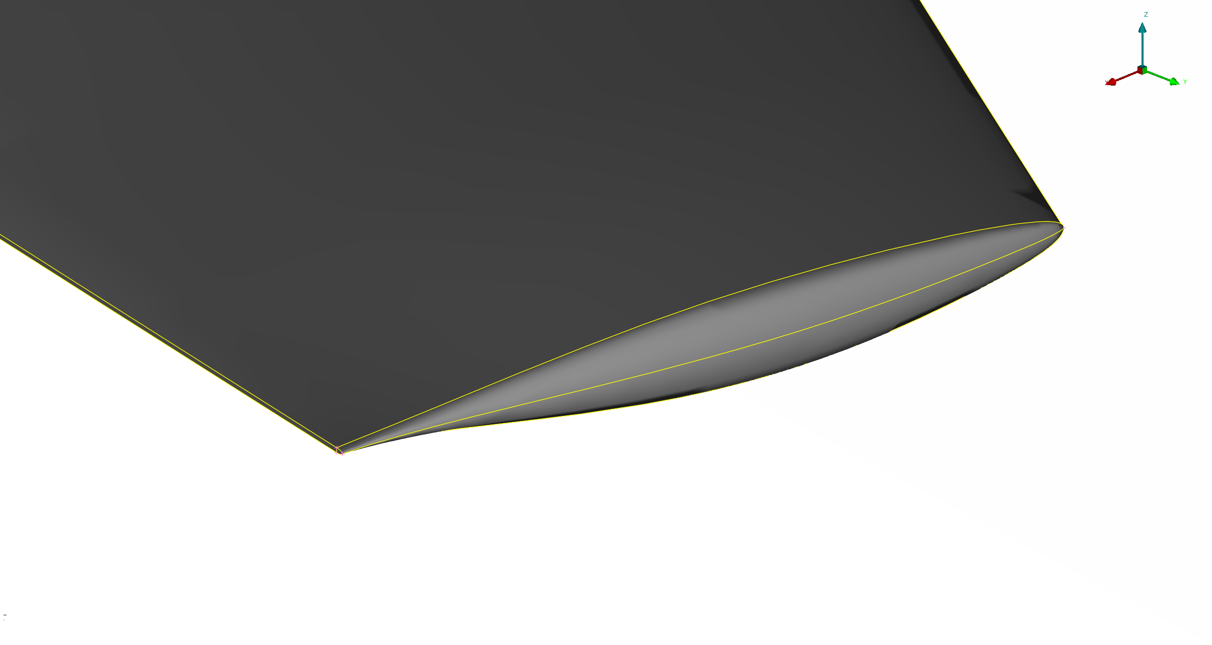
The cleaned master CAD file is shown below. Note that extra cuts have been added near the wing and tail caps to allow for ease of cap CAD separation.
Fuse Component
The fuse component has been cut out into two pieces which will become their own surfaces grids: the main body which has the holes left by the tail and wing removal filled, and the cap. Note that many of the extra lines of the master CAD have been removed. The only cuts which exist on the main body are those delineating curvature changes to allow for appropriate clustering. The nose has been inscribed with a square on the CAD instead of being drawn or grown on to simplify the surface definition. The fuse volumes have been grown out such that they adhere to the symmetry plane of the case.
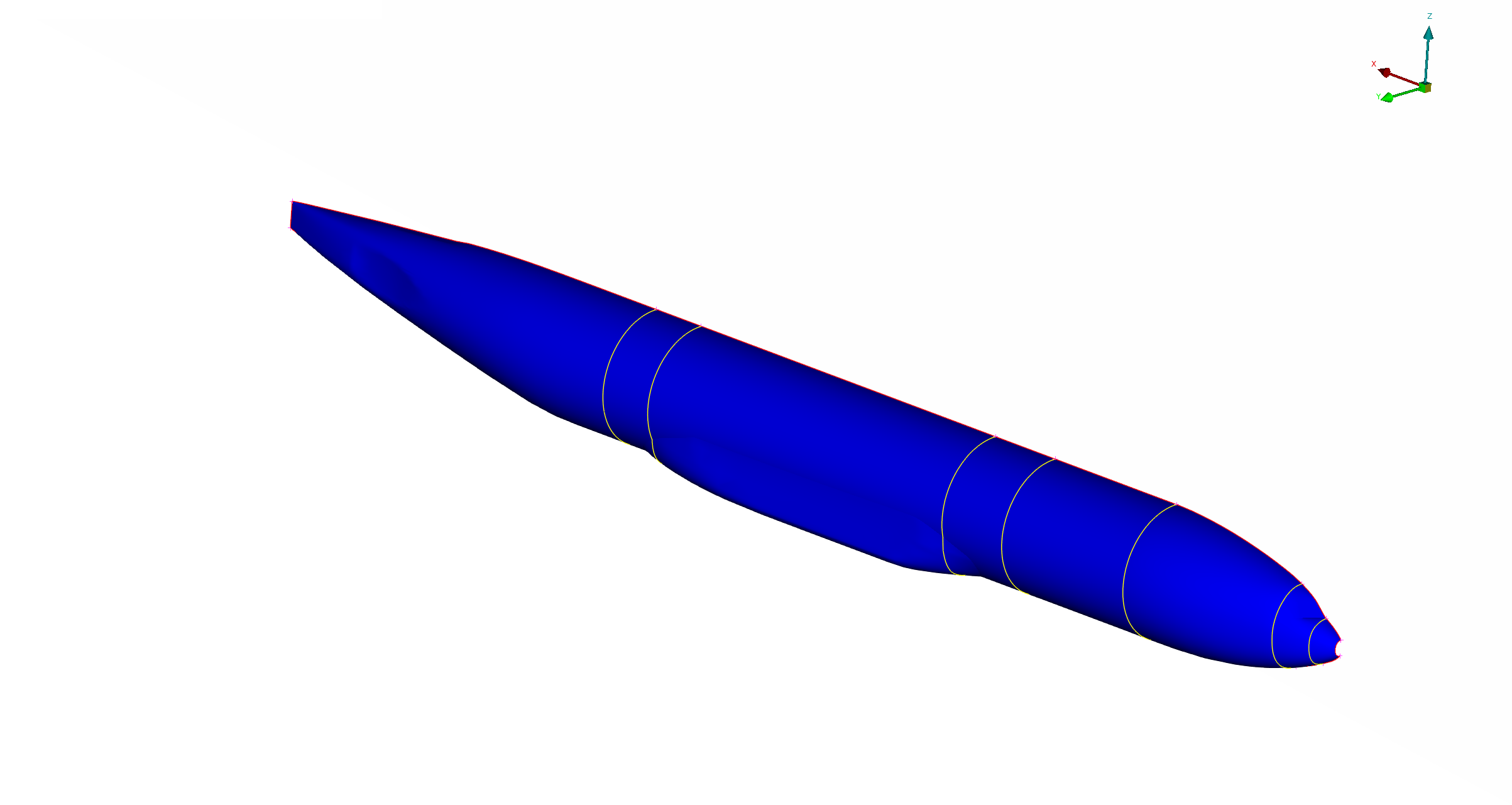
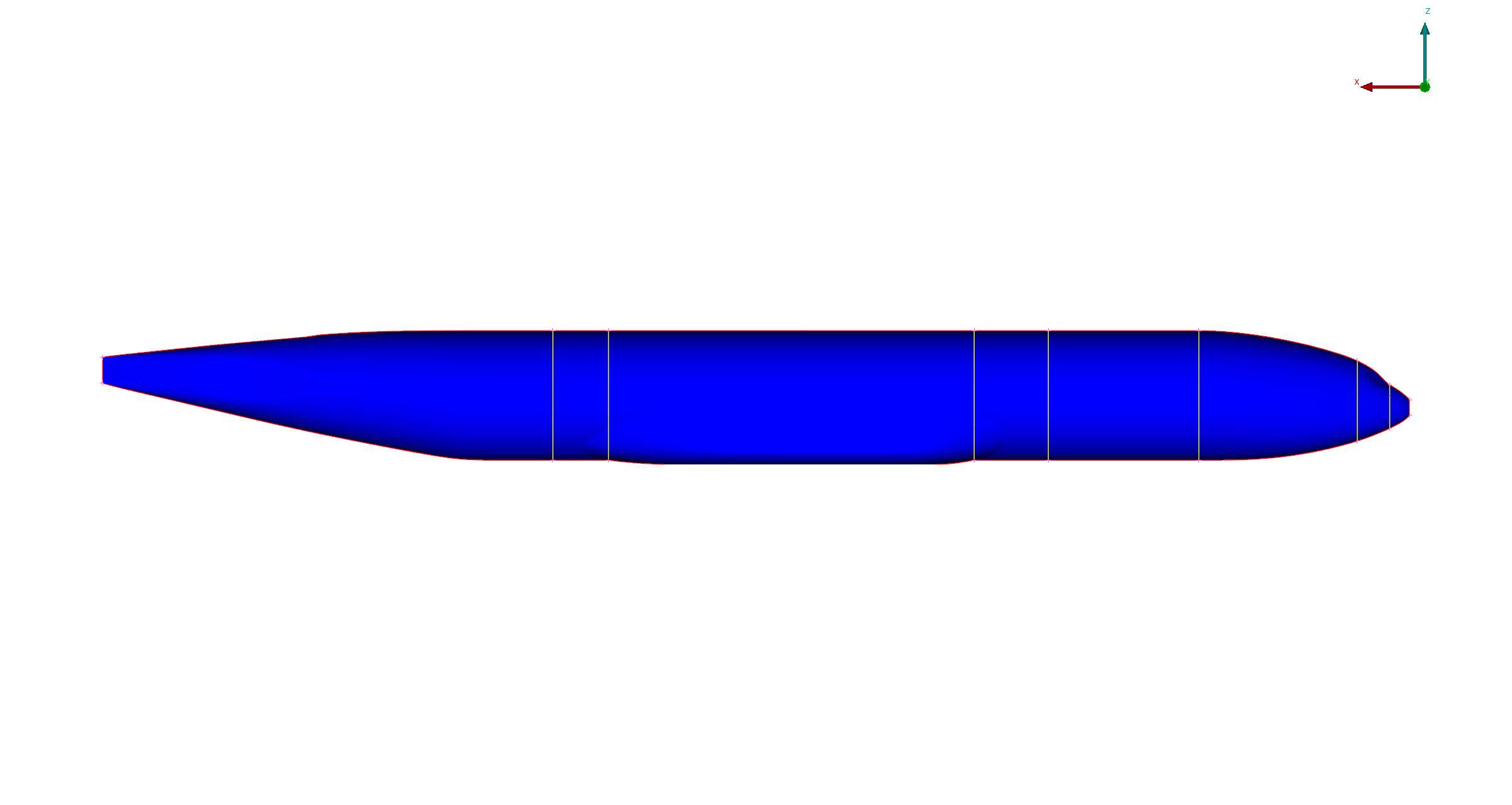
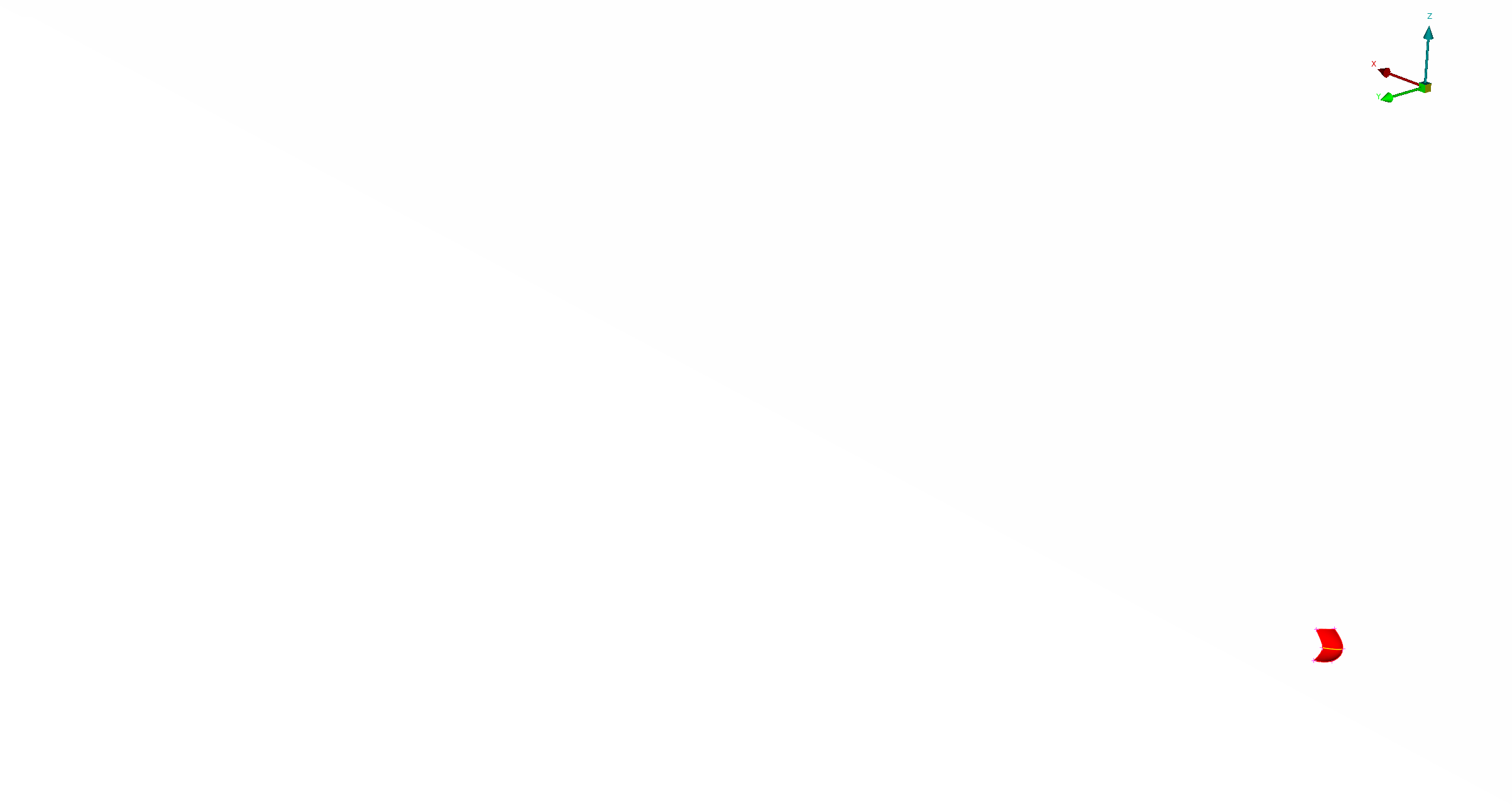
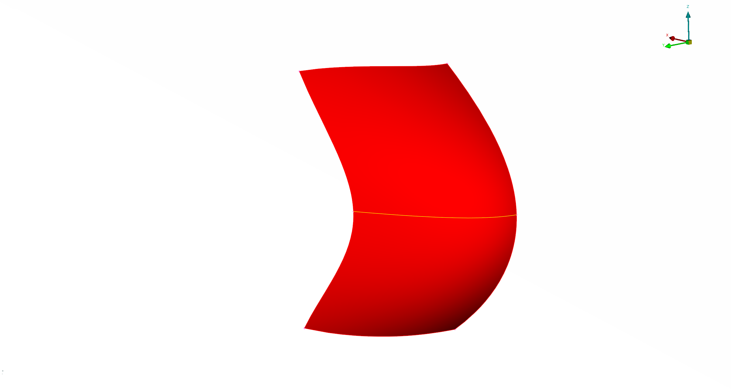
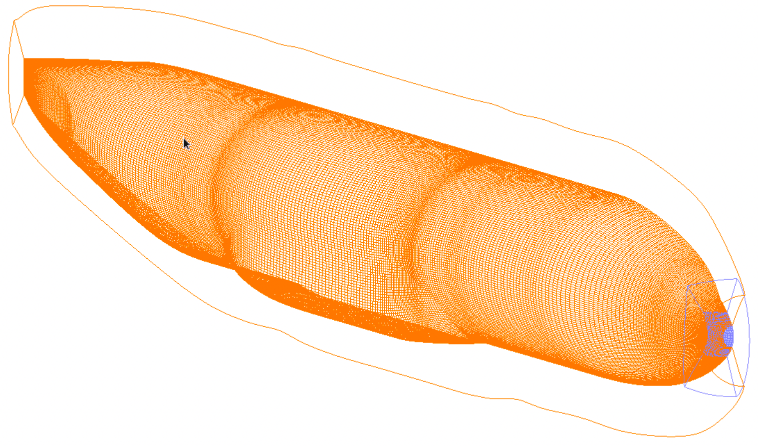
Lets take a look the portion of the 'fuse.tcl' script responsible for generating these volumes:
 73     # Use incremental building procedures (IBP).
 74     # --------
 75     IBP_initIncVars
 76     # --------
 77
 78     # The fuse body is grown along the symm plane except where it overlaps
 79     # with the nose.
 80     # --------
 81     puts "\tBuilding fuse body ..."
 82     # --------
 83     IBP_incVol
 84     # --------
 85     GenHypVolGrid FUSE_BODY.x v.[IBP_nVol] \
 86                   [list \
 87                       hyptan \
 88                       specsr \
 89                       $Par(sr) \
 90                       $Par(md) \
 91                       $Par(ds,wall) \
 92                       $Par(ds,glb) \
 93                       $Par(klayer) \
 94                   ] \
 95                   [list -10 2 2 2] \
 96                   [list 1.5 150 3]
 97     # --------
 98     IBP_extractBlkSurs v.[IBP_nVol] [list +L]
 99     # --------
100
101     # The nose has one side on the symm plane.
102     # --------
103     puts "\tBuilding fuse nose ..."
104     # --------
105     IBP_incVol
106     # --------
107     GenHypVolGrid FUSE_NOSE.x v.[IBP_nVol] \
108                   [list \
109                       hyptan \
110                       specsr \
111                       $Par(sr) \
112                       $Par(md) \
113                       $Par(ds,wall) \
114                       $Par(ds,glb) \
115                       $Par(klayer)\
116                   ] \
117                   [list -10 -10 2 -10] \
118                   [list 1.5 150 3]
119     # --------
120     IBP_extractBlkSurs v.[IBP_nVol] [list +L]
121     # --------
122
123     # Group the component meshes into surfaces and volumes.
124     # --------
125     IBP_combineGrids $fileN
126     # --------
The methodology for clean grid accounting utilized is 'incremental': the
surfaces and volumes are counted as new grids are made and then later combined,
such that only s.* (surface) and v.* (volume) files are created. They can
then later be deleted as a set without worry. IBP_initIncVars on line 75
instantiates the surface and volume counts. When a finished volume is created,
the volume count is first incremented (line 83), and then accessed through
[IBP_nVol] (line 85). The Par growth parameters of the volume are set in
MakeParm.tcl.
After each volume is created the sides of its block which are BCs are extracted
using IBP_extractBlkSurs on line 98 which takes a list of sides (+ being the
J, K, or L 1 side and - being the max side) and increments the surface count as
they are extracted. After all grids are built, the volumes and surfaces up to
the known count are combined on line 125.
You will see that the BC scripts use a similar method. The advantages of this
incremental style of building become more apparent when we look at more
complicated components such as the wing below, and also allow for extra grids
to be added in the middle of a script down the line without having to edit all
the variables below them. Below is an excerpt from fuse.BC.tcl in which the
following BC-addition functionality defined in
$LAVACGTToolsDir/AddBCInfoProcs.tcl is utilized for the body:
AddWallBCInfo $fileN [IBP_nVol] [list +L]       "fuse"
AddWallBCInfo $fileN [IBP_nVol] [list -J +K -K] "symm"
The AddWallBCInfo simply takes a grid index in the component and a list of
block sides and applies a BC name to it. The first says that the lMin side of
the fuse body is named 'fuse', while the jMax, kMin and kMax sides are
named 'symm'. We are not actually assigning BC types here for LAVA, only names:
the LAVA BC types are assigned in the yamls. There are delineations between
AddWall/Outlet/Etc/BCInfo proc calls in $LAVACGTToolsDir/AddBCInfoProcs.tcl
because a different file (bcmain.dat) is written by the master build script
which can be read into OVERGRID to visualize BCs, and that file needs to know
BC type.
Wing Component
The wing component consists of two overlapped CAD cutouts of the wing and its cap. The surface grids of the wing are pre-divided at feature lines that should be retained during the refinement procedure in a later tutorial. The Cap has a small surface at the trailing edge (TE) which is point-matched with the surfaces which loop around the cap tip.
Unlike the fuse, the wing has sharp feature lines which must be retained for the spline-and-refine procedures in a later tutorial. Thus, surface grids which are initially divided across feature lines are first interrogated for sizing, combined, and then grown out into a single volume which is re-divided. Doing this measurement within the scripts instead of hard-coding volume splitting numbers means that the surface grids can be freely altered and the grid scripts will still function as intended.
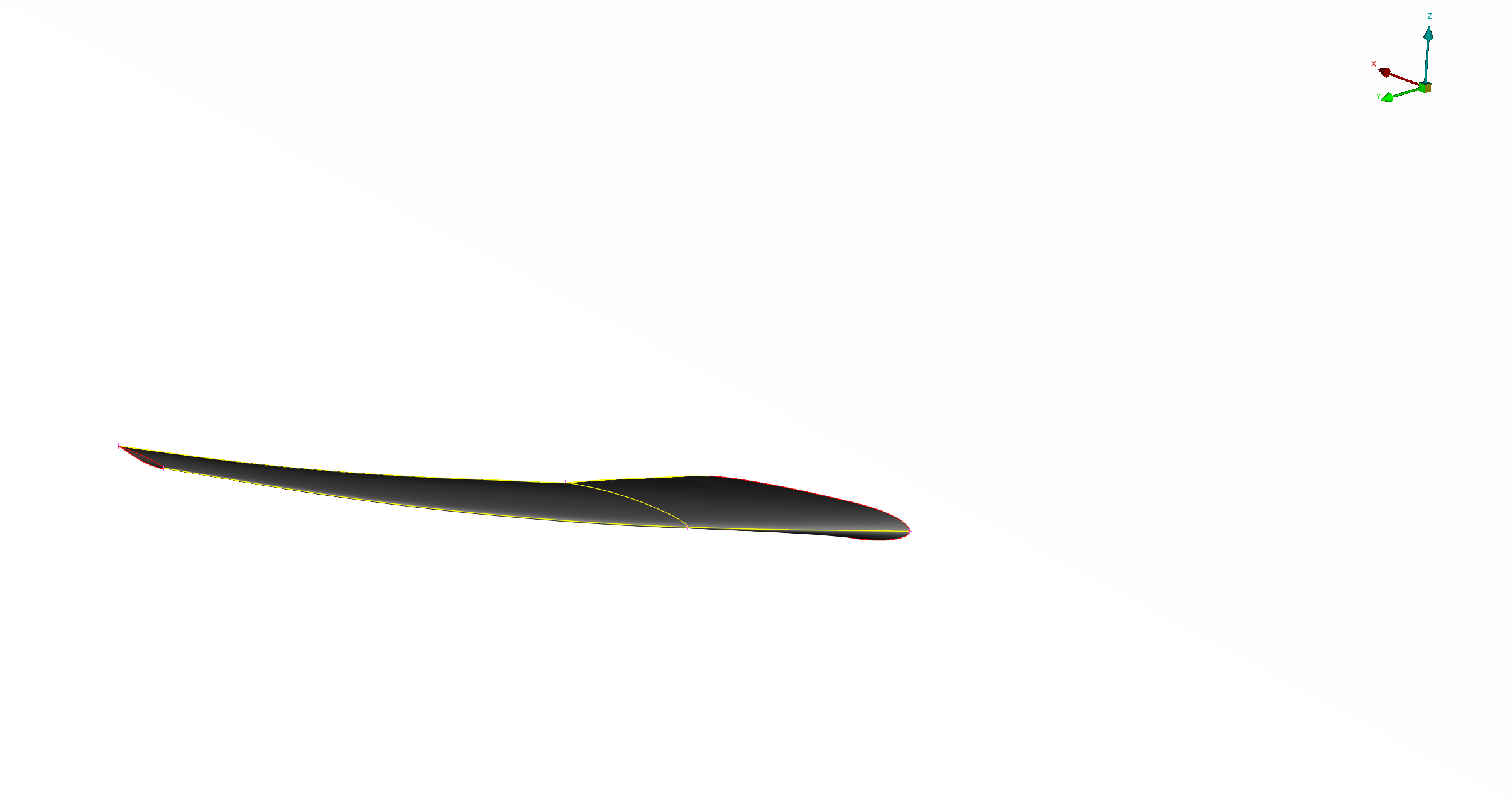
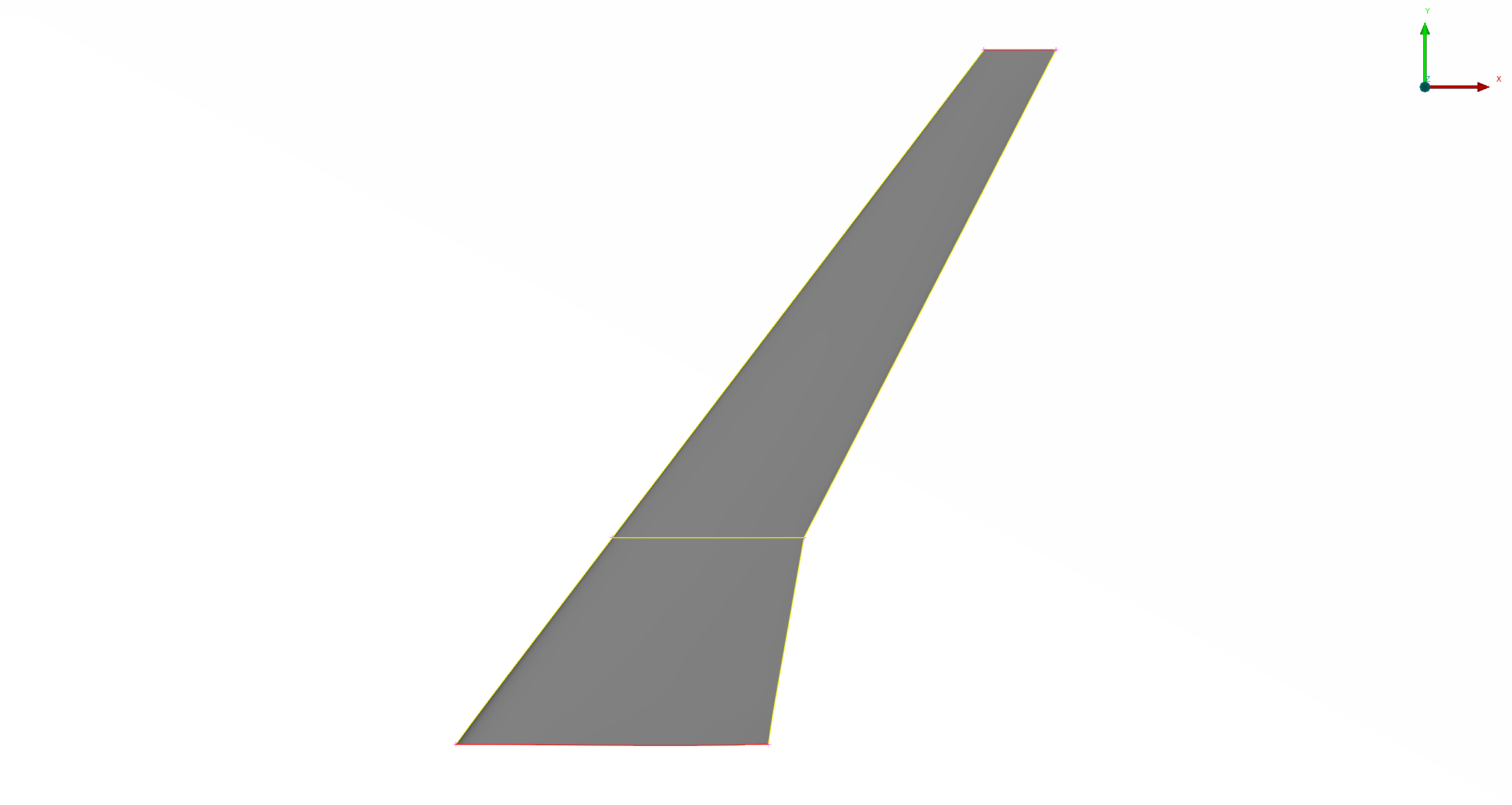
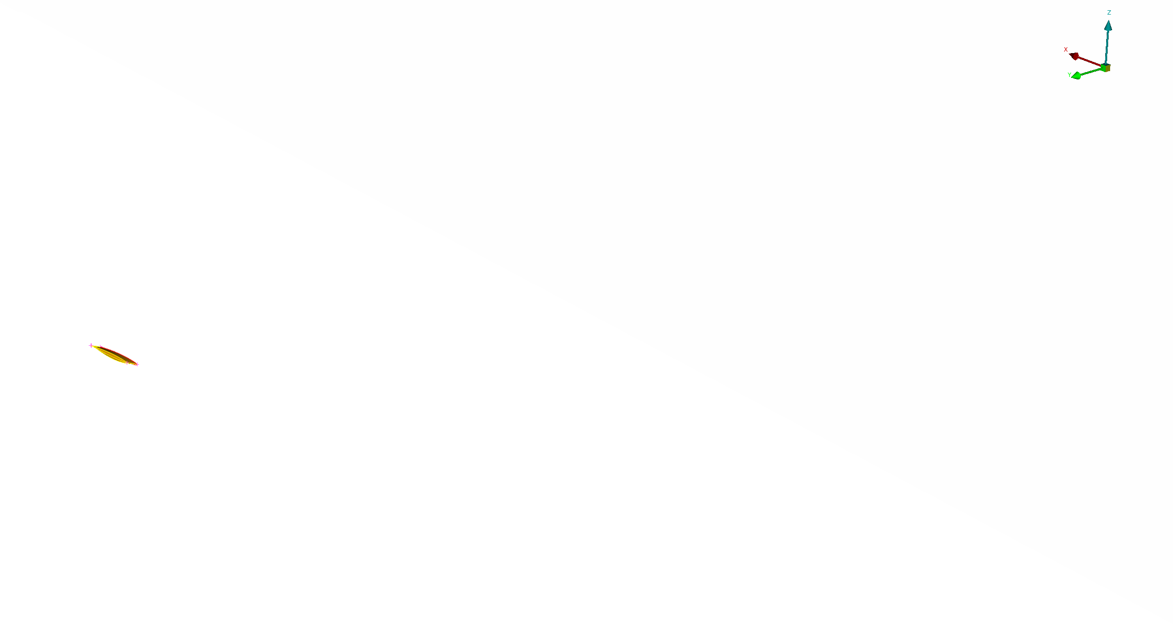
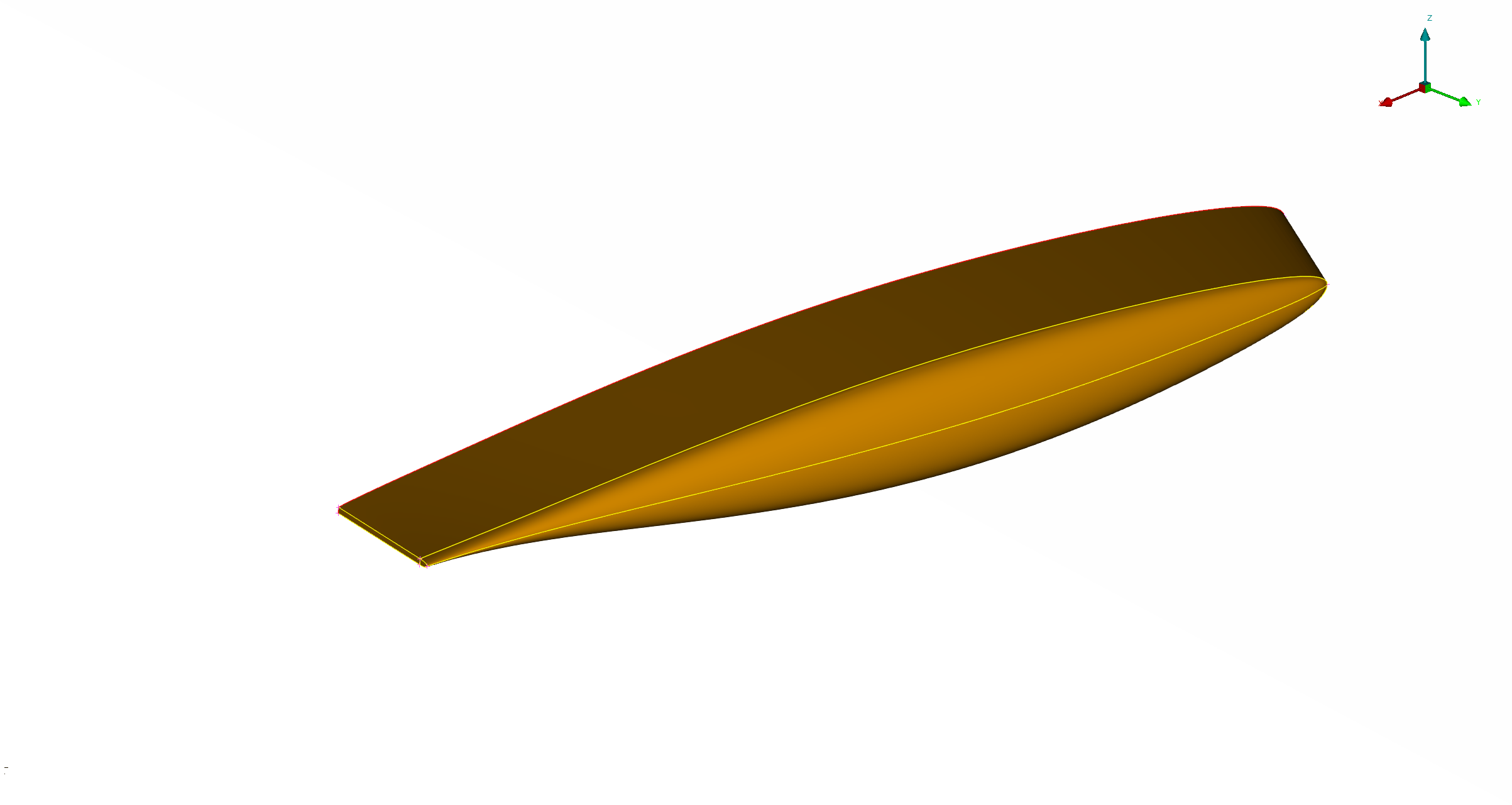
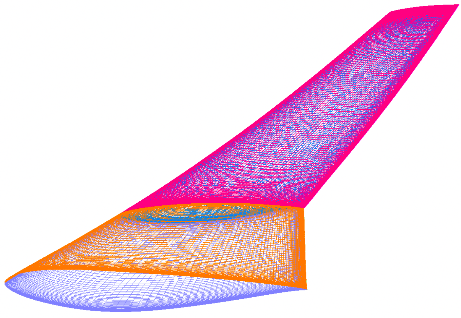
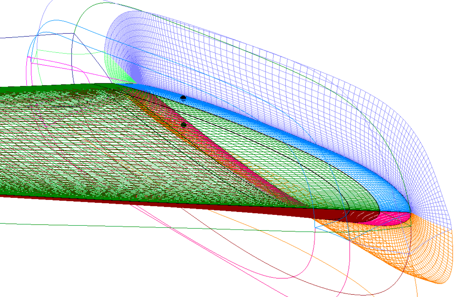
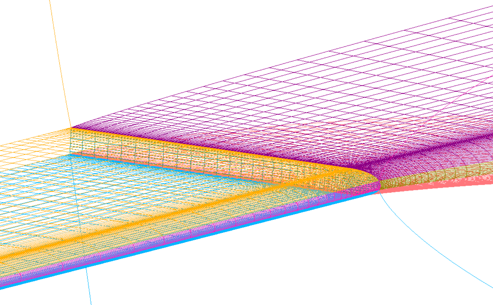
The junction between the wing and fuse is a collar constructed using the following code. A curve (denoted as c.*) extracted from the wing is projected onto the fuse, then grown onto it (lines 126-134). A portion of the wing surface is extracted and combined with the surface grown on the fuse (lines 135-138). A volume is generated and subsequently divided into 6 pieces.
The wing.tcl grid script better showcases the utility of incremental
building. The [IBP_nSurP 2] call on line 128 returns a number 2 higher than
the current surface count, preventing the user from accidentally overwriting a
previously made surface. The volume constructed in line 139 calls [IBP_nVolP
7], to give room for the six feature line-respecting volumes which are
subsequently extracted from it. While the collar is built first in this script,
this code chunk could technically be pasted anywhere in the file and it would
still function as intended. This same strategy is used for the wing itself.
126     ExtractSubs    WING_WING.x c.1 [list 1 1 -1 1 1 1 1]
127     Project        c.1 fuse.sur dummy c.2 [list -1] [list 1] [list 1 n 0 0 1]
128     GenHypSurGrids fuse.sur c.2 s.[IBP_nSurP 2] 1 1 \
129                    [list \
130                        -1 \
131                        [list 10 10] \
132                        [list 25 0 0.05 0.000263 0.0] \
133                        [list 0.5 20] \
134                    ]
135     SwapInd        s.[IBP_nSurP 2] s.[IBP_nSurP 1] [list revj revk]
136     ExtractSubs    WING_WING.x s.[IBP_nSurP 2] \
137                    [list 1 1 -1 2 [expr $wingColEndK + $Par(np,hlfOrlp)] 1 1]
138     ConcatGridsn   [list s.[IBP_nSurP 1] s.[IBP_nSurP 2]] s.[IBP_nSurP 3] k 0
139     GenHypVolGrid  s.[IBP_nSurP 3] v.[IBP_nVolP 7] \
140                    [list \
141                        hyptan \
142                        specsr \
143                        $Par(sr) \
144                        $Par(md) \
145                        $Par(ds,wall) \
146                        $Par(ds,glb) \
147                        $Par(klayer)\
148                    ] \
149                    [list 10 10 -20 -20] \
150                    [list 1.5 250 3]
The cap grids of the wing demonstrate one strategy to create a set of grids at the TE which are well-aligned with flow coming off the wing. As shown on lines 293-298 below, a copy of the small TE cap grid is translated aft of the wing, connected to the one still on the wing TE, and then re-distributed to generate a volume grid which matches the spacing of the other cap grids on the wing surface in the stream-wise direction.
293     IBP_incVol
294     # --------
295     GedTranslate WING_CAP_TE.x s.[IBP_nSurP 1] $teTx $teTy $teTz
296     ConcatGridsn [list WING_CAP_TE.x s.[IBP_nSurP 1]] v.[IBP_nVolP 1] l 0
297     SrapRedist   v.[IBP_nVolP 1] v.[IBP_nVol] 1 l 1 2 0 \
298                  [list 1 -1 $Par(sr) $teDs 0.0]
The surfaces of this cap TE volume are then extracted and combined with those cap surfaces on the wing abutting the TE (lines 315-323). The combined surface is then grown as one volume which will subsequently be re-divided to six volumes which respect the TE feature lines as was done with the wing and collar before (lines 324-335).
315     ExtractSubs   v.[IBP_nVol] s.[IBP_nSurP 2] [list 1  1 -1  1  1  1 -1]
316     SwapInd       s.[IBP_nSurP 2] s.[IBP_nSurP 1] [list swaplk swapjk revk]
317     ExtractSubs   v.[IBP_nVol] s.[IBP_nSurP 3] [list 1  1  1  1 -1  1 -1]
318     SwapInd       s.[IBP_nSurP 3] s.[IBP_nSurP 2] [list swaplj]
319     ExtractSubs   v.[IBP_nVol] s.[IBP_nSurP 4] [list 1  1 -1 -1 -1  1 -1]
320     SwapInd       s.[IBP_nSurP 4] s.[IBP_nSurP 3] [list swaplk swapjk]
321     ConcatGridsn  [list s.[IBP_nSurP 1] s.[IBP_nSurP 2] s.[IBP_nSurP 3]] \
322                   s.[IBP_nSurP 4] k 1
323     ConcatGridsn  [list WING_CAP_OUT.x s.[IBP_nSurP 4]] s.[IBP_nSurP 1] j 1
324     GenHypVolGrid s.[IBP_nSurP 1] v.[IBP_nVolP 7] \
325                   [list \
326                       hyptan \
327                       specsr \
328                       $Par(sr) \
329                       $Par(md) \
330                       $Par(ds,wall) \
331                       $Par(ds,glb) \
332                       $Par(klayer) \
333                   ] \
334                   [list -10 -1 -5 -5] \
335                   [list 1.5 150 3]
Tail Component
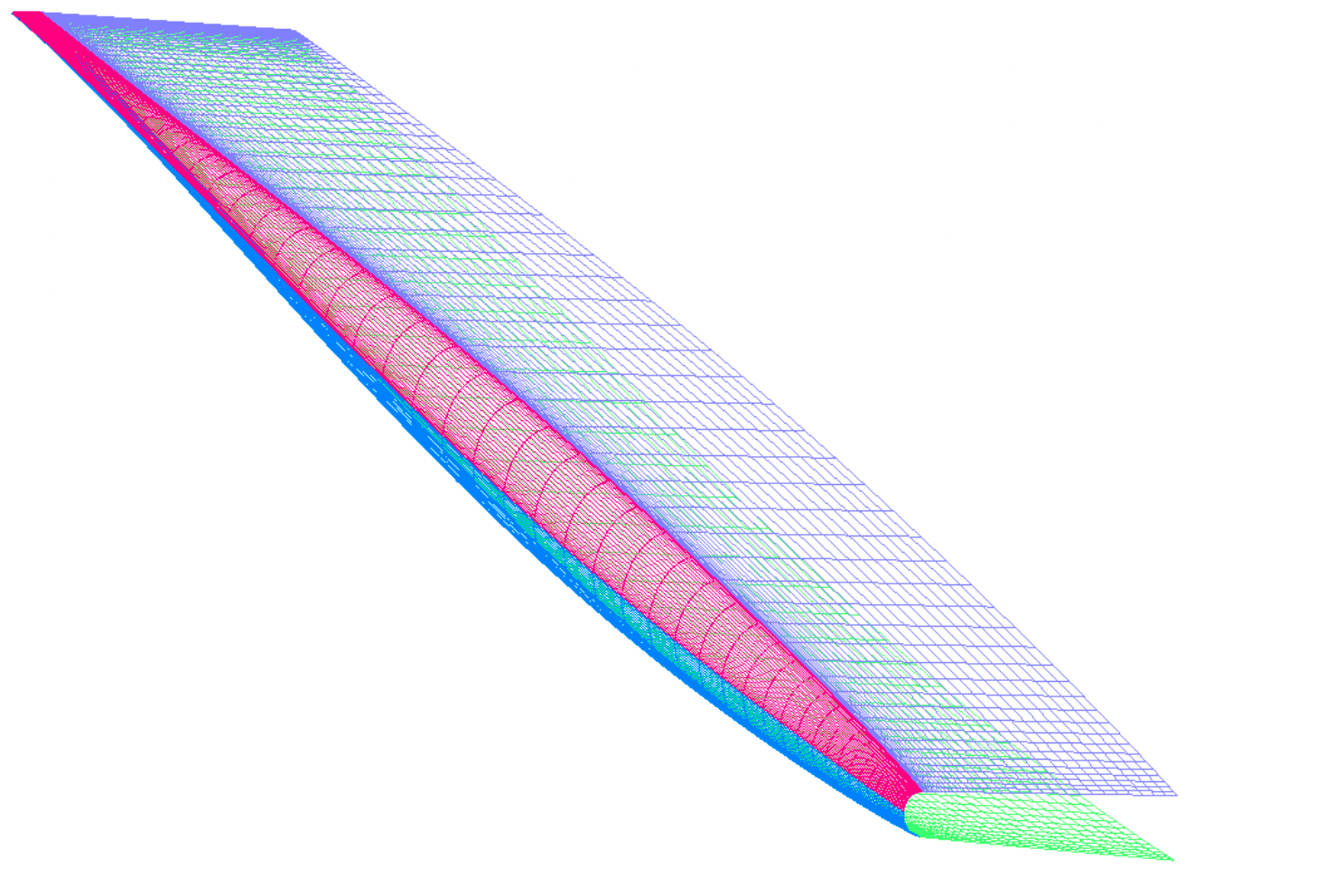
The tail component uses the same methodology as the wing for its collar with the fuse and its body. Its cap, however, showcases a different construction method.
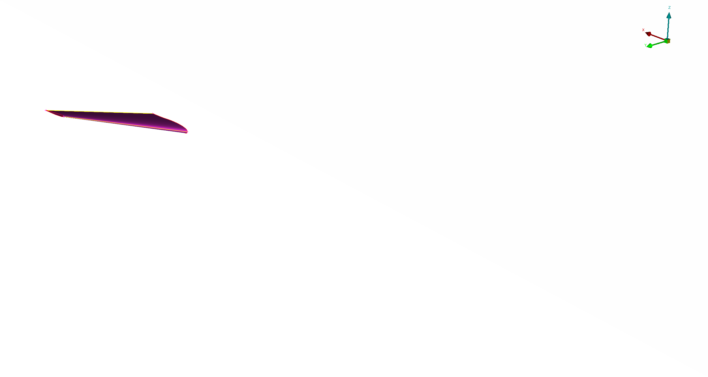
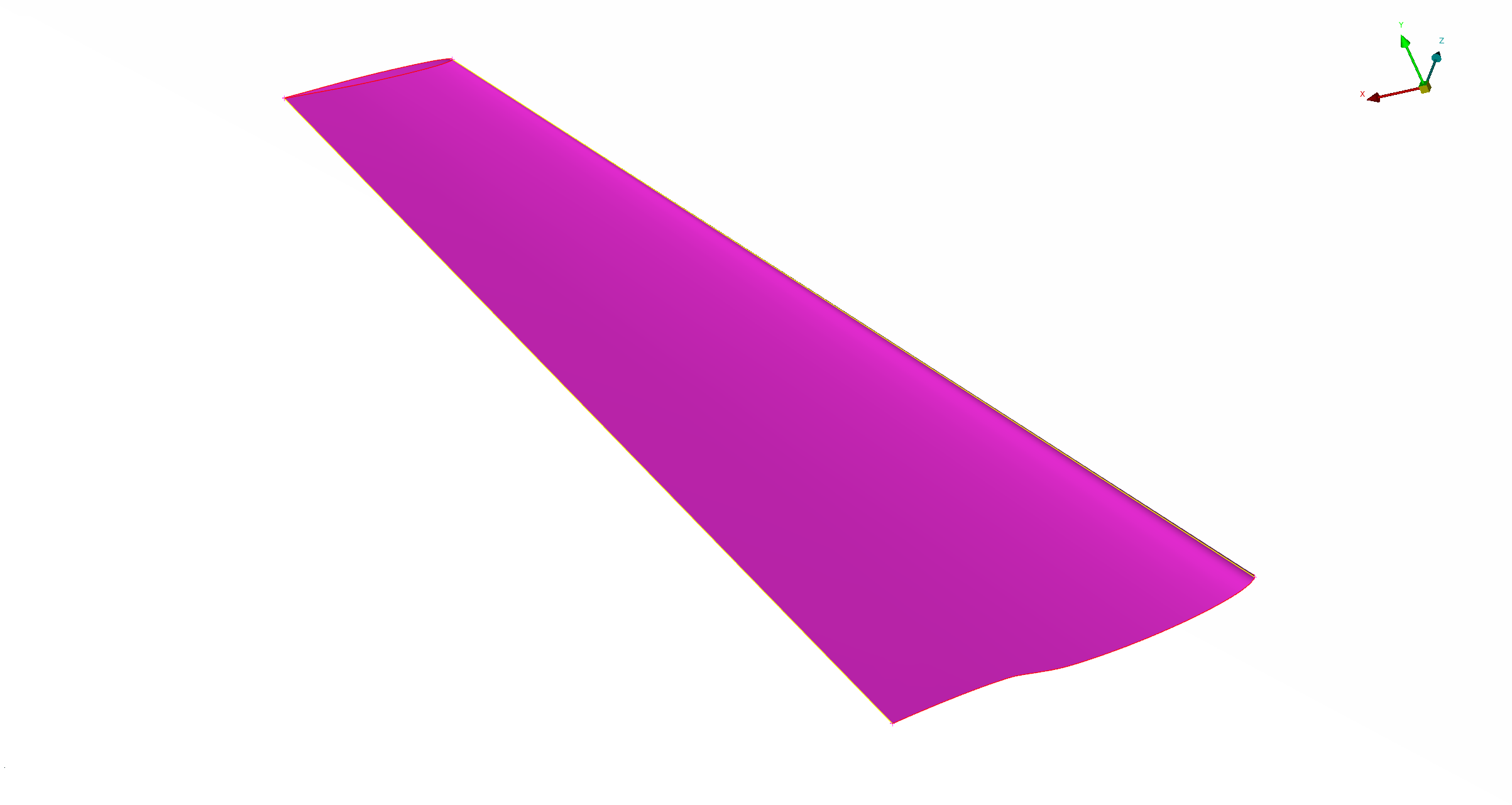
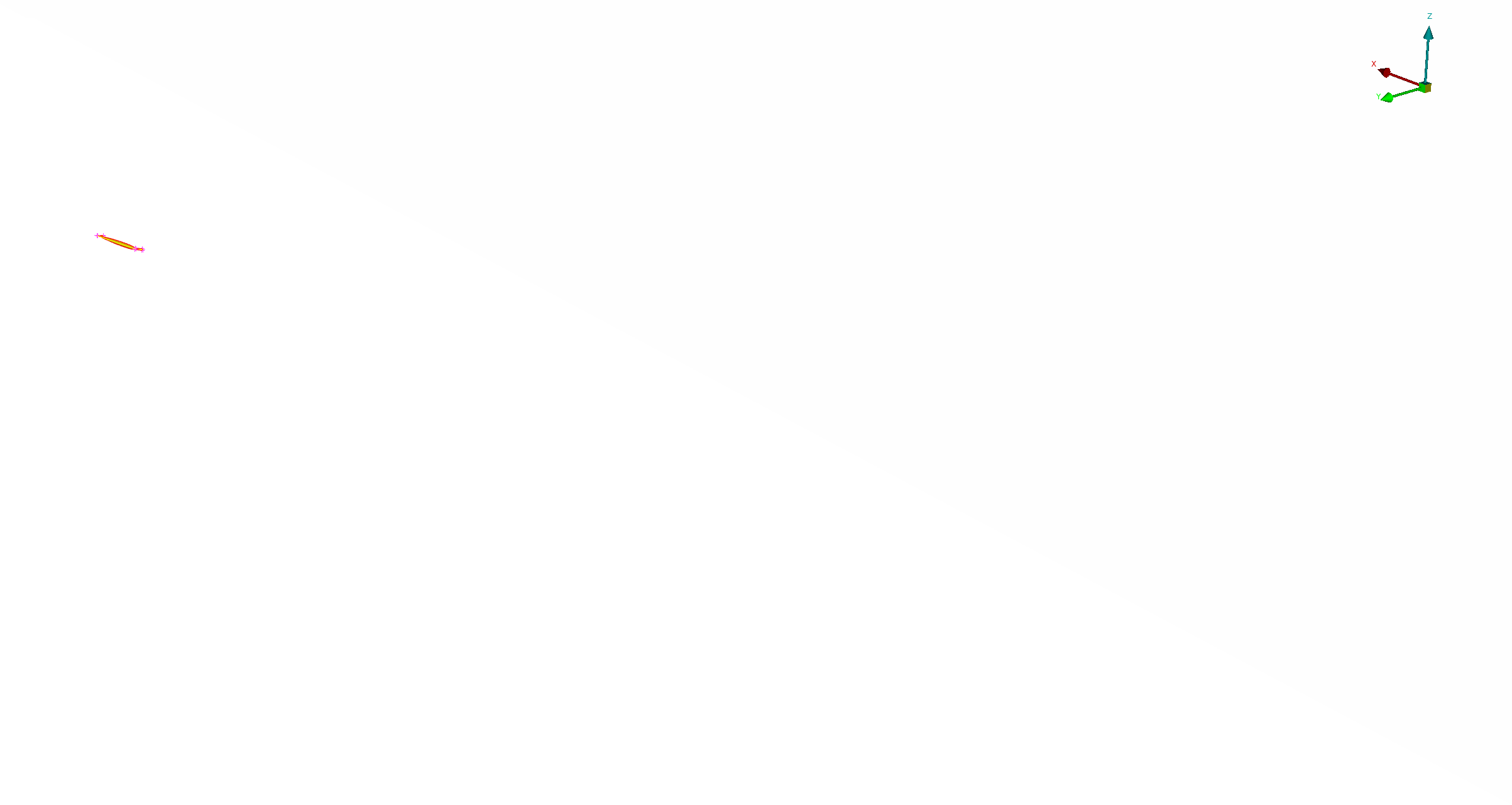
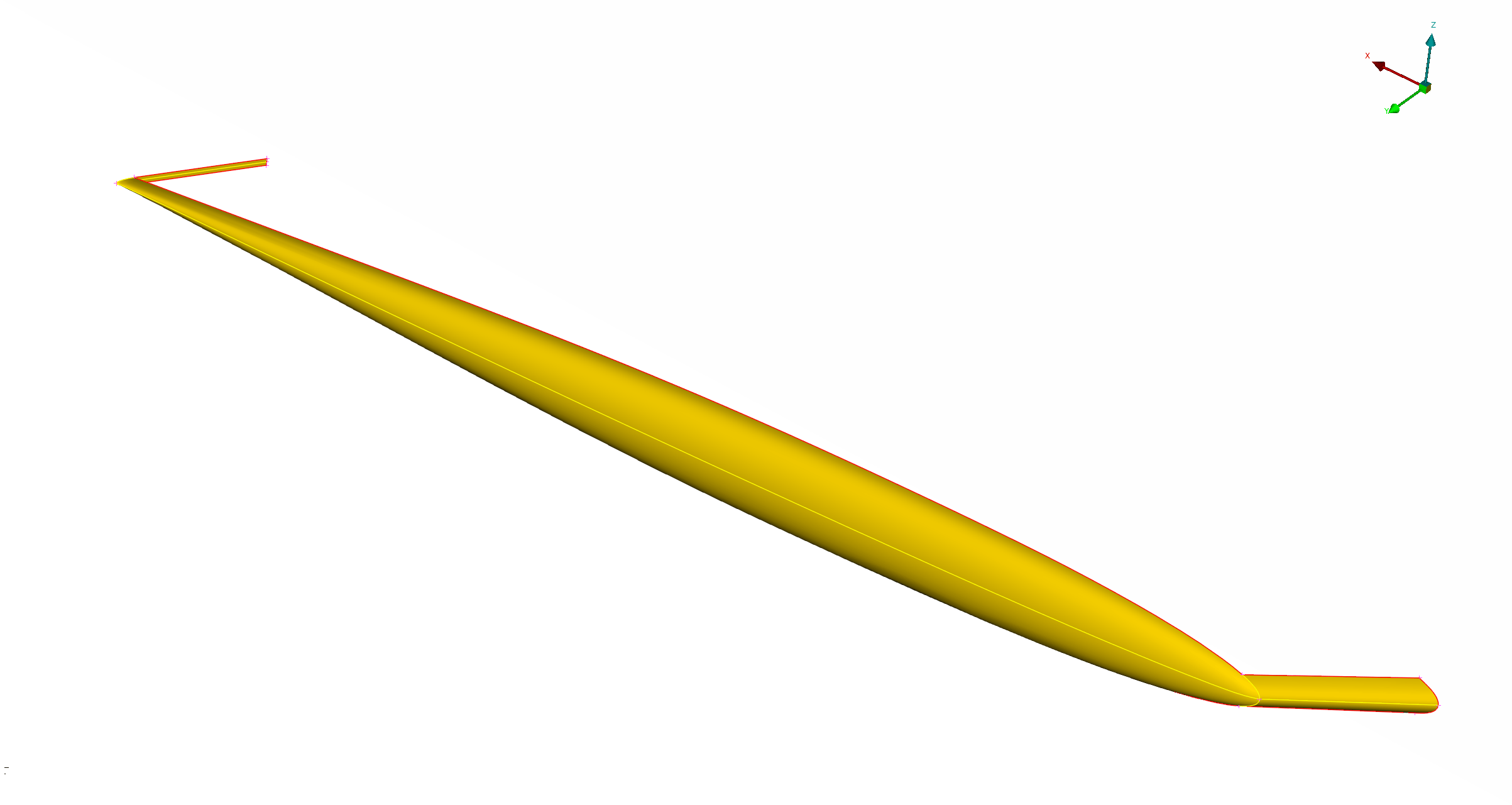
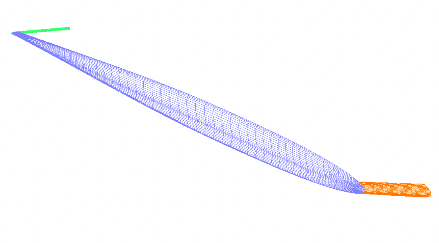
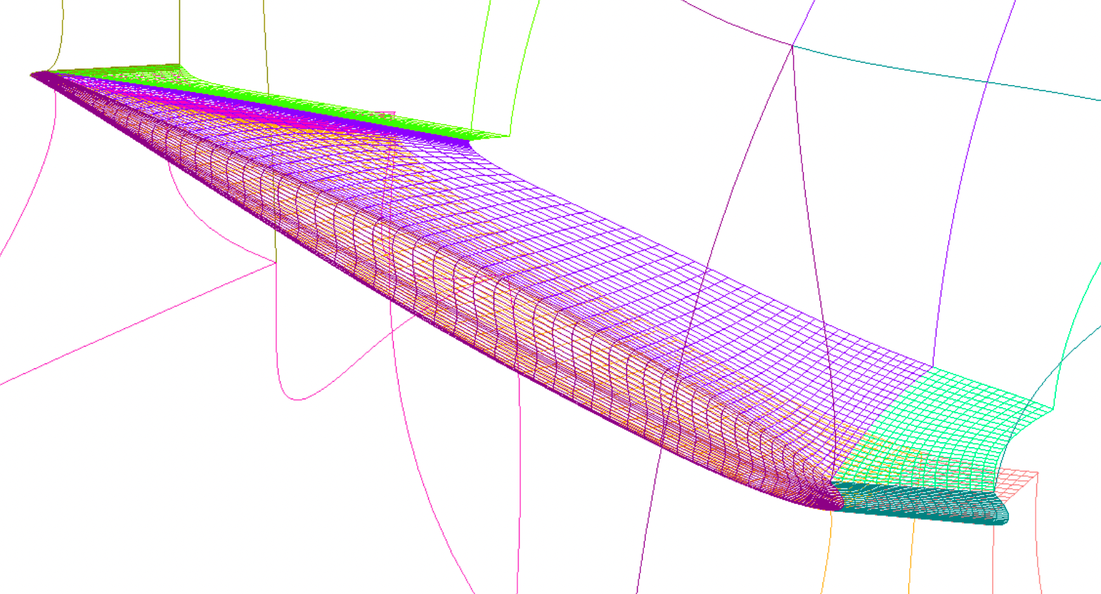
The tail cap surfaces are initially defined on outer mould lines of the cap
only, and not on the wing itself. The cap surfaces were initially divided into
leading, outer, and trailing edges, but were measured and combined at the start
of the tail.tcl script. The curve of the combined grid on the tail top is
extracted, projected onto a triangular surface representing the local tail, and
then grown along it (lines 267-277). The same is then done for the tail bottom
(lines 281-290). Finally, the grids are combined and grown as one volume, which
will be subsequently split into the 9 volumes shown above (lines 293-306).
267     ExtractSubs    TAIL_CAP.x c.2 [list 1 1 -1 1 1 1 -1]
268     ReverseInd     c.2 c.1 [list revj]
269     Project        c.1 TAIL_REF.i.tri dummy c.2 [list -1] [list -1] \
270                    [list 1 n 0 0 1]
271     GenHypSurGrids TAIL_REF.i.tri c.2 s.[IBP_nSurP 2] 1 1 \
272                    [list \
273                        1 \
274                        [list -1 -20] \
275                        [list 25 0 0.01 0.0002 0.0] \
276                        [list 5.0 150 0.0 3] \
277                    ]
278     ReverseInd     s.[IBP_nSurP 2] s.[IBP_nSurP 1] [list revj revk]
279     set nKCapTop   [lindex [GetDim s.[IBP_nSurP 1] 1] 1]
280     # --------
281     ExtractSubs    TAIL_CAP.x c.1 [list 1 1 -1 -1 -1 1 -1]
282     Project        c.1 TAIL_REF.i.tri dummy c.2 [list -1] [list -1] \
283                    [list 1 n 0 0 1]
284     GenHypSurGrids TAIL_REF.i.tri c.2 s.[IBP_nSurP 2] 1 1 \
285                    [list \
286                        1 \
287                        [list -1 -20] \
288                        [list 25 0 0.01 0.0002 0.0] \
289                        [list 5.0 150 0.0 3] \
290                    ]
291     set nKCapBot   [lindex [GetDim s.[IBP_nSurP 2] 1] 1]
292     # --------
293     ConcatGridsn  [list s.[IBP_nSurP 1] TAIL_CAP.x s.[IBP_nSurP 2]] \
294                   s.[IBP_nSurP 3] k 1
295     GenHypVolGrid s.[IBP_nSurP 3] v.[IBP_nVolP 10] \
296                   [list \
297                       hyptan \
298                       specsr \
299                       $Par(sr) \
300                       $Par(md) \
301                       $Par(ds,wall) \
302                       $Par(ds,glb) \
303                       $Par(klayer) \
304                   ] \
305                   [list -20 -20 -20 -20] \
306                   [list 0.5 5 1]
Building the CRM Project Grid
You will note that the grid.* files constructed with
buildProjectGrid_nearBody.tcl do not constitute a closed computational
domain, i.e. a far-field or off-body grid set doesn't exist. While there are
ways to create such far-field grids using CGT scripting, LAVA provides an
octFarfield executable which makes a size-efficient resolution-telescoping
Cartesian box-grid set given a closed surface triangulation to target as the
smallest telescoped grid level. The triangulated surface generated from the
masterCAD.igs file (NEARBODY_REF.plt) which will be used is shown below.
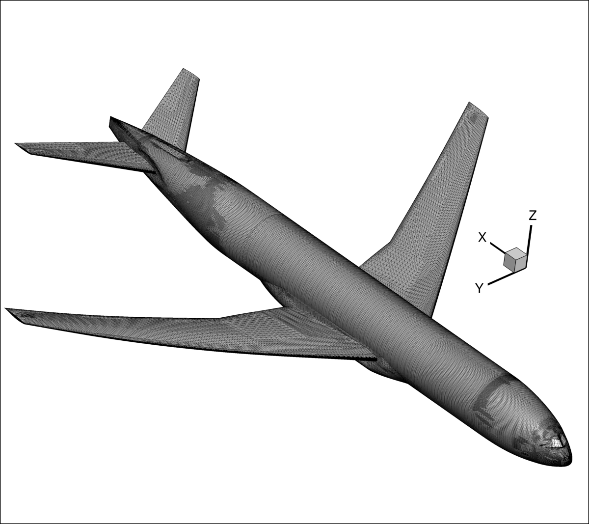
Using this executable is not possible within the CGT scripting framework
described above, as it should be threaded and has its own input yaml file.
Thus, to conjoin the nearBody scripting-generation method and offBody
exe-generation method we utilize the run_buildGrid.sh bash script, shown
below. Remember to properly set the LAVACGTToolsDir, LAVA_EXE_DIR,
LAVA_EXE_SUFFIX, and OMP_NUM_THREADS environmental variables in
envVars.sh first.
# Build the nearBody grid using the normal project build script.
# By default the grid is built to grid.in: renaming here is just preference
# becuase we will be combining this grid with the exe-generated farField grid.
# ---------------------------------------------------------------------------- #
baseDir=$( cd -- "$( dirname -- "${BASH_SOURCE[0]}" )" &> /dev/null && pwd )

source $baseDir/envVars.sh

$baseDir/buildProjectGrid_nearBody.tcl

mv -f grid.in    nearBodyGrid.x
mv -f grid.bc.in nearBodyGrid.bc
mv -f grid.sur   nearBodyGrid.sur
mv -f grid.b2b   nearBodyGrid.b2b
mv -f bcmain.dat nearBodyGrid.bcmain.dat
rm -f gridnames.txt
# ---------------------------------------------------------------------------- #

# Build the farField using the octFarfield exe.
# First copy over the input script and the surface representation it requires
# as a starting point.
# ---------------------------------------------------------------------------- #
cp $baseDir/geom/NEARBODY_REF.plt .
cp $baseDir/auxFiles/LAVA_octFarField.yaml .

$LAVA_EXE_DIR/octFarfield.$LAVA_EXE_SUFFIX LAVA_octFarField.yaml

rm NEARBODY_REF.plt LAVA_octFarField.yaml check.plt farFieldGrid.x.cart
# ---------------------------------------------------------------------------- #

# use the mergeGrids exe guild combine the nearBody and farField -> final grid.
# The 'surface' grid is defined simply as the nearbody surface grid.
# ---------------------------------------------------------------------------- #
$LAVA_EXE_DIR/mergeGrids.$LAVA_EXE_SUFFIX nearBodyGrid.x farFieldGrid.x grid.x

cp -f nearBodyGrid.sur grid.sur
# ---------------------------------------------------------------------------- #
The nearBody CGT generation master script buildProjectGrid_nearBody.tcl is
called first. The offBody generation is conducted next after the appropriate
files needed by the executable are copied over. Finally, the two grids and
their BCs are combined. The LAVA_octFarField.yaml far-field generation input
file is shown below. dx determines the grid spacing in [m] which should
encompass the nearBody triangulation. cubeLength determines the total size of
the far-field limits, which is adjusted by how many times the farField is
expected to telescope its grid resolution (nRefine). The symmetry plane has
been enforced in the outerBCs. More information on the octFarField yaml
arguments can be found in the curvilinear documentation.
octFarField:
  inputType :             surface
  inputFileType :         tecplot
  inputFile :             NEARBODY_REF.plt
  externalFlow :          True
  dx :                    0.006
  ymin :                  0.0
  cubeLength :            200.0
  outerBCs :              [far, far, symm, far, far, far]
  nRefine :               16
  nCellBuffer :           24
  nbuffer :               0
  usenearbodycoarsening : False
  outputName :            farFieldGrid
  includeoverlap :        True
The resulting files are grid.x and grid.bc, which are the required input to
the connectivity process discussed in the next tutorial. Views of the
farFieldGrid.x and zoomed-in grid.x are shown below.
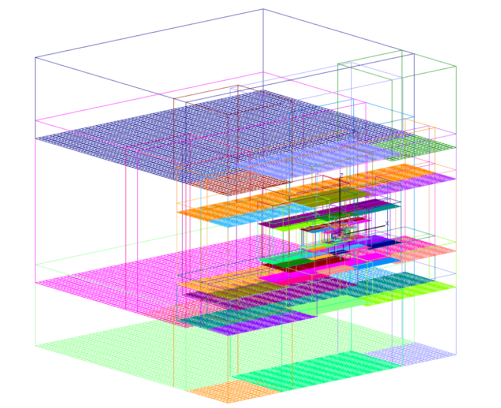
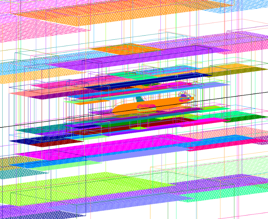
The nearBody grid has 40 grids and ~125 million nodes, while the farField grid has 161 grids and ~118 million nodes, for a combined set of 201 grids with ~243 million nodes.