Including Immersed Geometry
Immersed boundaries are a feature within the lavacurv solver which allows
portions of the computational domain to have a momentum penalty term applied,
effectively enforcing a wall-body-like effect on the flow if the penalty term
is strong enough. Immersed triangulated surfaces are supplied in the input
yaml, and all nodes within them are tagged as immersed. There can be multiple
surfaces and they can all have settings (see the immersedBoundaries yaml
settings).
Application of immersed boundaries is utilized mainly for two purposes:
- There are small shapes which are annoying to grid and only their downstream/bluff-body effects matter.
- There are components which intersect with other components in a manner which makes collar grid generation challenging and time consuming.
For the former purpose, a small uniformly spaced immersion box can be placed into the grid system and the immersed surface will introduce an approximation of the shape.
For the latter, we likely want comparable flow physics to be introduced by the immersed effects as a viscous wall BC, as well as integrated loads. In this case, we seek to produce 'body-fitted' immersion grids which both conform to the immersed surface as well as possible, AND have viscous wall spacing at the immersed boundary surface.
In this tutorial we will be adding a body-fitted flow-through nacelle to the body-wing-tail CRM, then using a body-fitted immersed pylon to connect it to the wing.
Body-Fitted Immersed Component Scripting
There are many strategies for scripting body-fitted immersion grids. The general idea though is to start with the fewest or simplest surface grids on portions of the immersed geometry which will be touching the fluid. Grids on the surface will be grown both inward and outward from the immersed surface so that there is viscous spacing on both sides of the immersed surface. Similarly to regular body-fitted grids, the better these grids represent the curvature of your immersed boundary the better its representation and thus your solution will be.
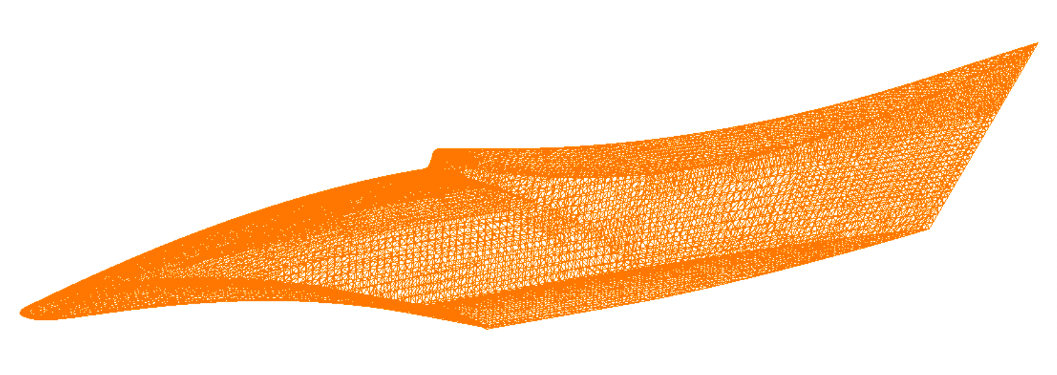
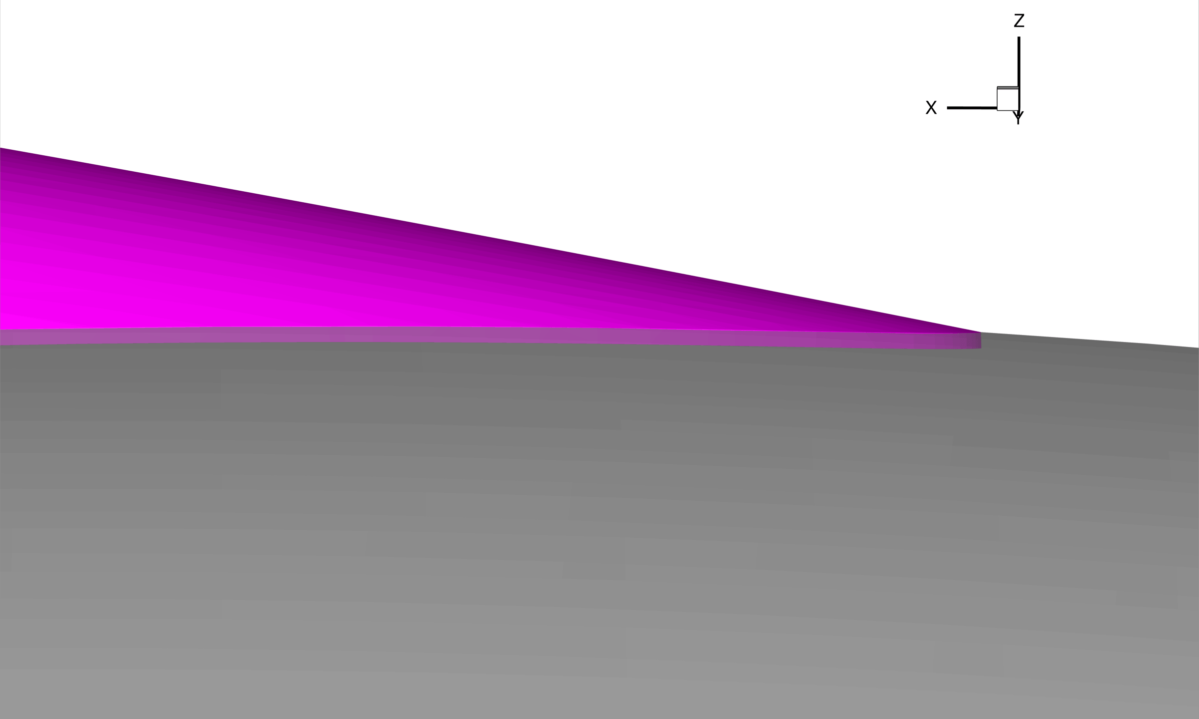
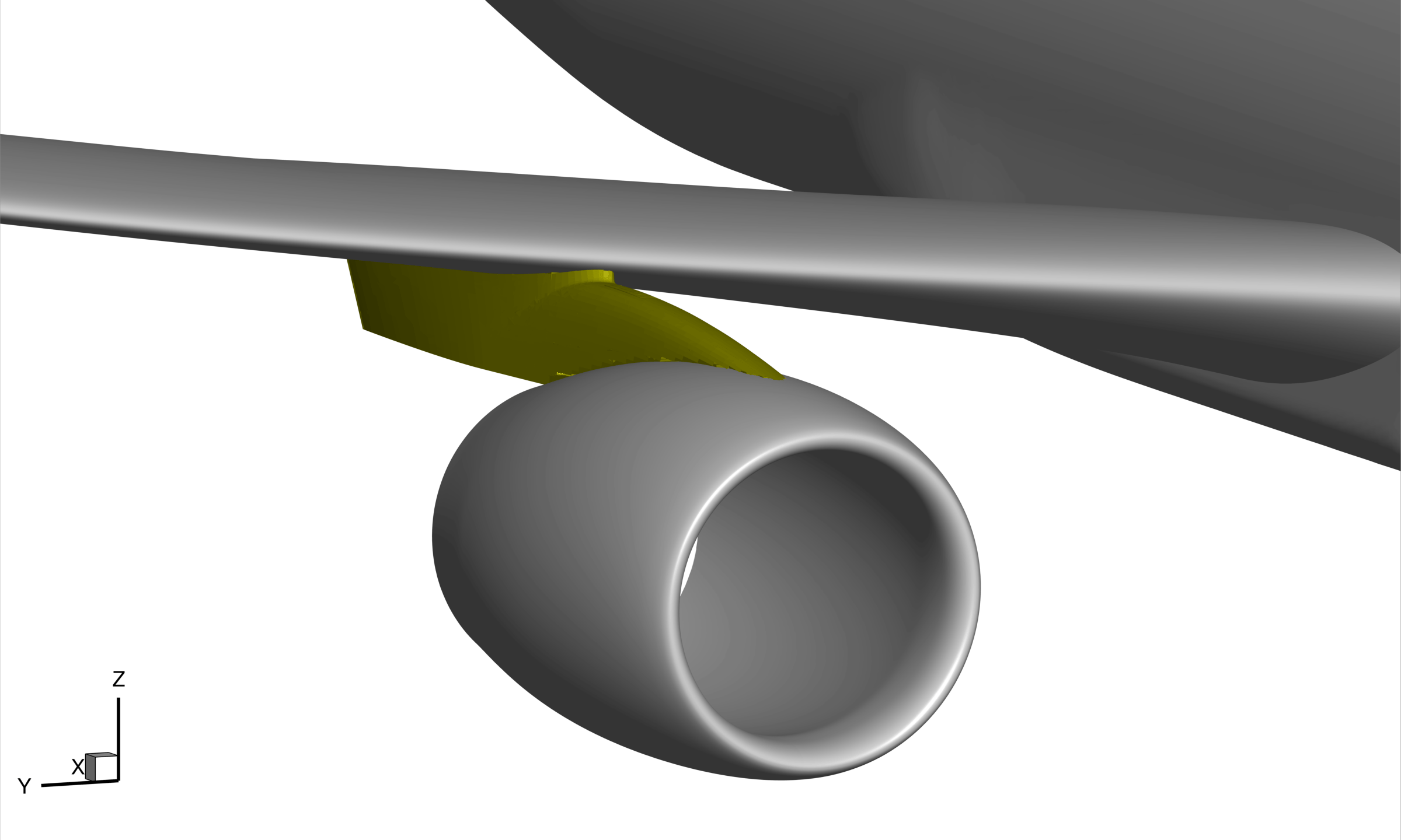
The pylon's immersed surface triangulation is shown below.
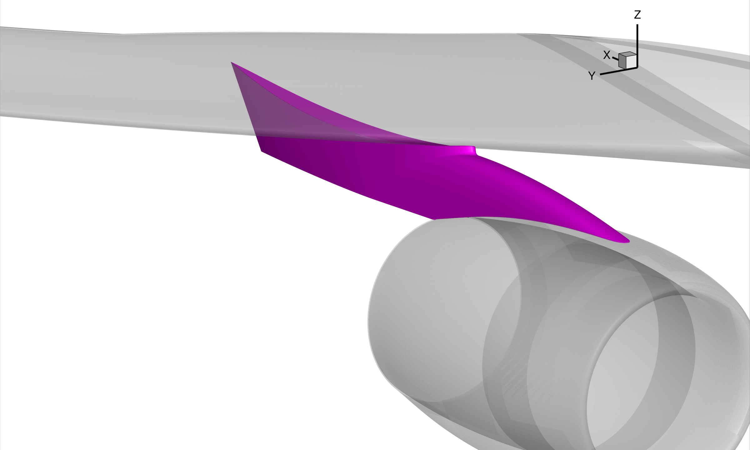
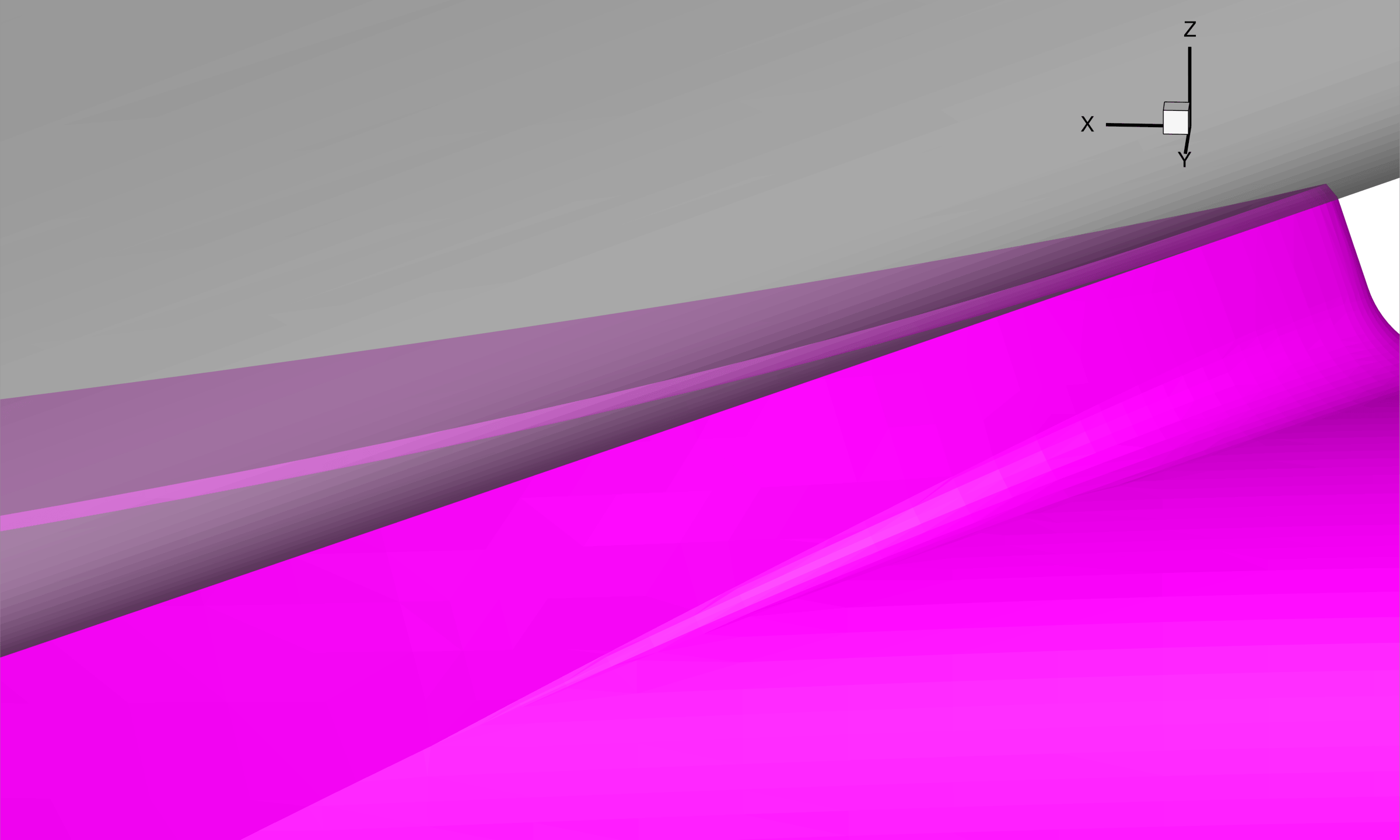
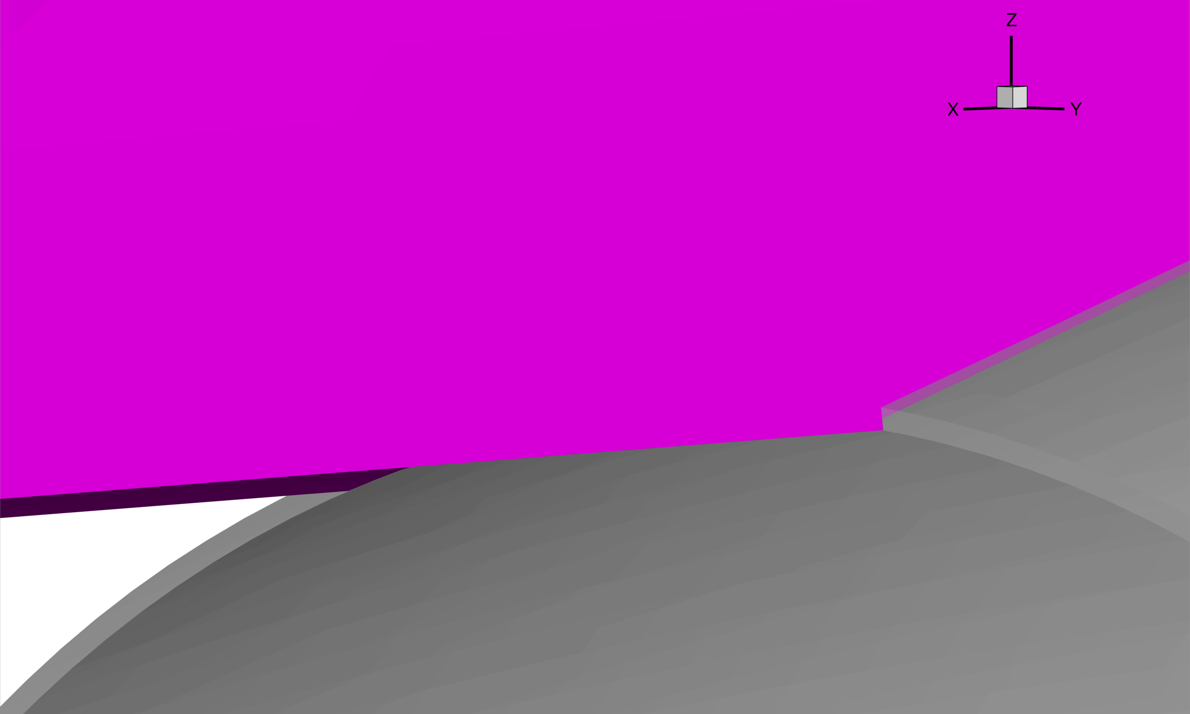
The CAD this surface was built on was slightly extruded to extend into the wing and pylon bodies, as seen below. Without these proper intersections, integrated loads and immersed boundary enforcement won't be correct at the components' intersections.
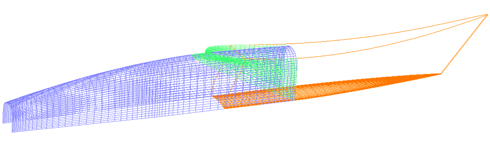
When considering this immersed surface, several factors influenced the initial choice of grids, which are shown below.
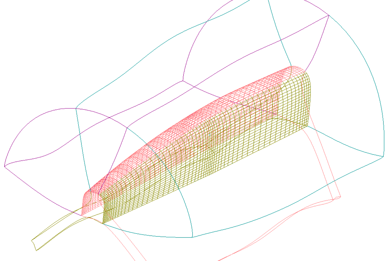
- The 'aft' grid (orange) fills the aft region of the pylon, and intersects with the wing component. This will be extended out from the pylon in a doubly-viscous manner. When the internals of the surface are square-like this is a good option since extension outward is easily script-able, and better fills the internal space than growing inward on all sides.
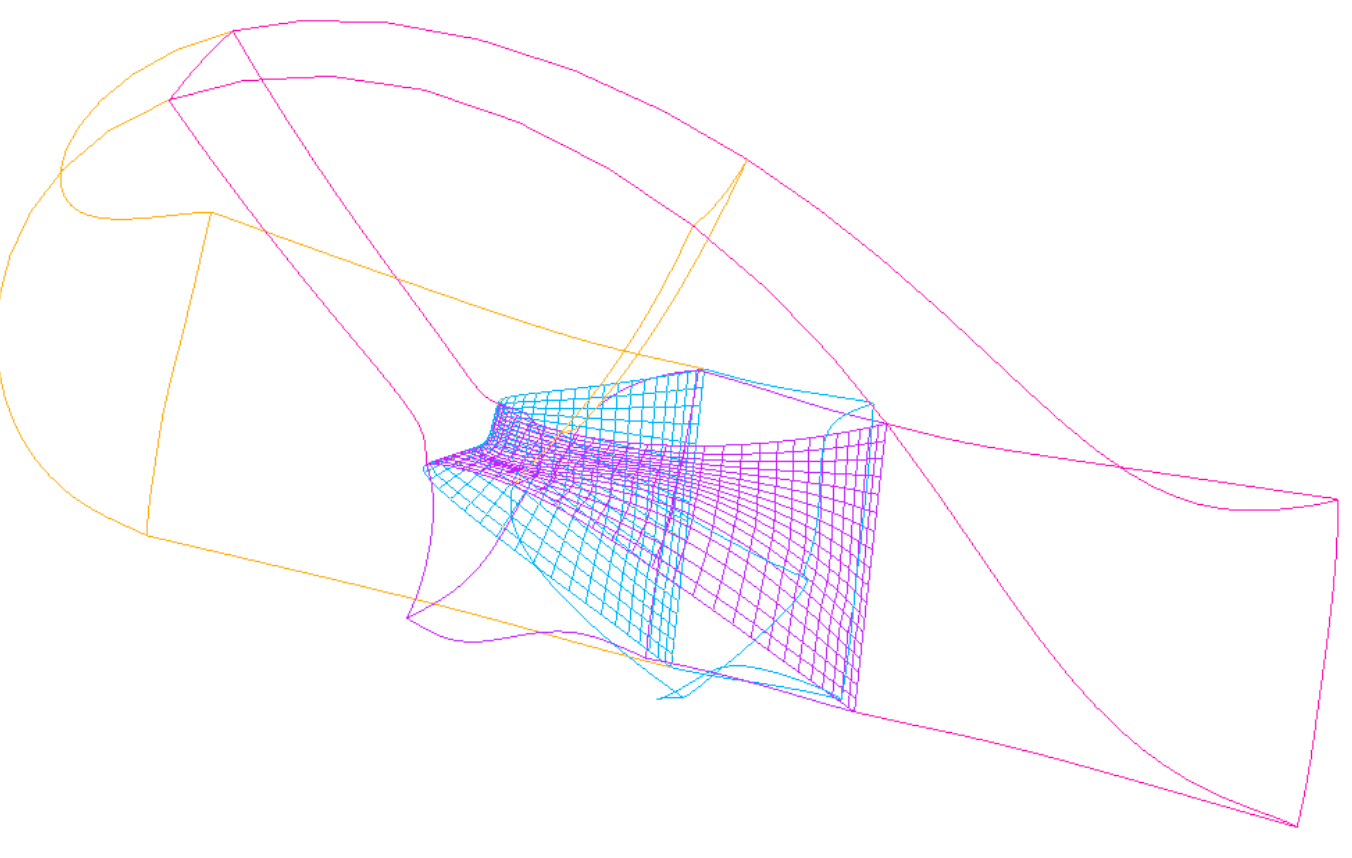
- The 'nose' grid (blue) handles the intersection with the nacelle. We don't care about what happens at the 'bottom' of the immersed surface's nose because it will be inside the nacelle geometry. We will grow inward and outward from the nose top. Grids grown inward here will just be optimized out during connectivity if they pass through the nacelle.
- The 'cusp' grid (green) is similar to the nose, but has been separated in order to prevent the nose from being hard to hyperbolically grow. Feel free to make many easy to create/grow patches on immersed surfaces to reduce grid scripting iterations.
The scripted building process for the pylon's aft section begins with re-distributing the internal aft block to be viscous in all directions but stream: we do not need to resolve the trailing edge with viscous spacing.
set npVisc 65
SrapRedist PYLON_AFT.x     v.[IBP_nVolP 1] 1 -k 1 1 0 \
           [list 1 -1 $npVisc $Par(ds,wall) $Par(ds,wall)]
SrapRedist v.[IBP_nVolP 1] v.[IBP_nVolP 2] 1 -l 1 1 0 \
           [list 1 -1 $npVisc $Par(ds,wall) $Par(ds,wall)]
We then repeatedly take one of the sides of the block, orient it to grow in the direction of our choice, grow it, then recombine it with the original block. Below is that process with the trailing edge side (jMax), and outboard side (kMax), but this is subsequently performed with kMin, and finally lMin. Note that the TE is translated, concatenated and redistributed, while the outboard is grown to make the grown cells more uniform. The bottom (lMin side) is translated, redistributed and concatenated to get a smoothed effect more manually because it is not well posed for hyperbolic growth.
# TE
# --------
ExtractSubs  v.[IBP_nVolP 2] s.[IBP_nSurP 1] [list 1 -1 -1  1 -1  1 -1]
GedTranslate s.[IBP_nSurP 1] s.[IBP_nSurP 2] \
             0.0685153964825696 0.002566620622606264 -0.001506420730025947
ConcatGridsn [list s.[IBP_nSurP 1] s.[IBP_nSurP 2]] v.[IBP_nVolP 1] j 0
SrapRedist   v.[IBP_nVolP 1] v.[IBP_nVolP 3] 1 j 1 5 0 \
             [list 1 -1 $Par(sr) $dsJEndAftBdy $Par(ds,glb) $Par(ds,glb)]
ConcatGridsn [list v.[IBP_nVolP 2] v.[IBP_nVolP 3]] v.[IBP_nVolP 1] j 1
# --------
# Outboard side.
# --------
ExtractSubs   v.[IBP_nVolP 1] s.[IBP_nSurP 1] [list 1  1 -1 -1 -1  1 -1]
SwapInd       s.[IBP_nSurP 1] s.[IBP_nSurP 2] [list swapkl revk]
GenHypVolGrid s.[IBP_nSurP 2] v.[IBP_nVolP 2] \
              [list \
                  hyptan \
                  specsr \
                  $Par(sr) \
                  $Par(md) \
                  $Par(ds,wall) \
                  $Par(ds,glb) \
                  $Par(klayer) \
              ] \
              [list -2 -2 -2 -2] \
              [list 1.5 150 3]
SwapInd       v.[IBP_nVolP 2] v.[IBP_nVolP 3] [list swapkl revl]
ConcatGridsn  [list v.[IBP_nVolP 1] v.[IBP_nVolP 3]] v.[IBP_nVolP 2] k 1
# --------
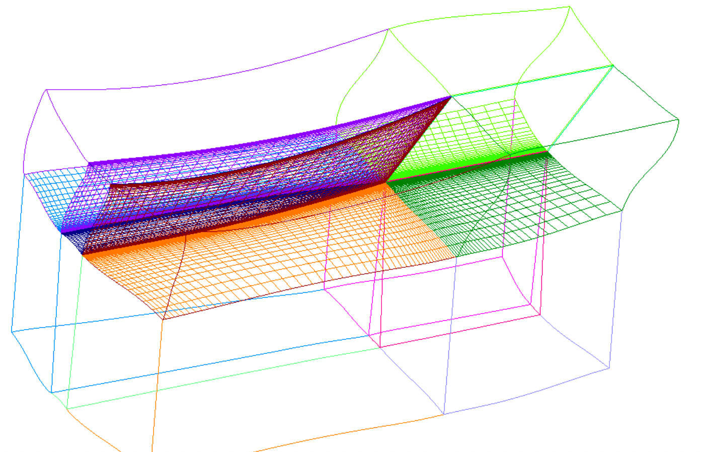
Once the final extended block has been created, the volumes can be pulled out using grid delineation counts found during the extension process, as shown below for the first two of the 12 aft grids. These blocks are re-oriented so that their lMin sides lie 'on' the immersed boundary to more intuitively see its shape in overgrid.
puts "\tBuilding pylon aft ..."
# --------
IBP_incVol
# --------
ExtractSubs PYLON_AFT.x v.[IBP_nVolP 1] \
            [list 1           1 $npJAftBdy \
                              1  $npKAftIn \
                              1 $npLAftBot]
SwapInd     v.[IBP_nVolP 1] v.[IBP_nVol] [list revl swapk]
# --------
IBP_incVol
# --------
ExtractSubs PYLON_AFT.x v.[IBP_nVolP 1] \
            [list 1  $npJAftBdy         -1 \
                              1  $npKAftIn \
                              1 $npLAftBot]
SwapInd     v.[IBP_nVolP 1] v.[IBP_nVol] [list revl swapk]
# --------
The final aft volume set is shown below.
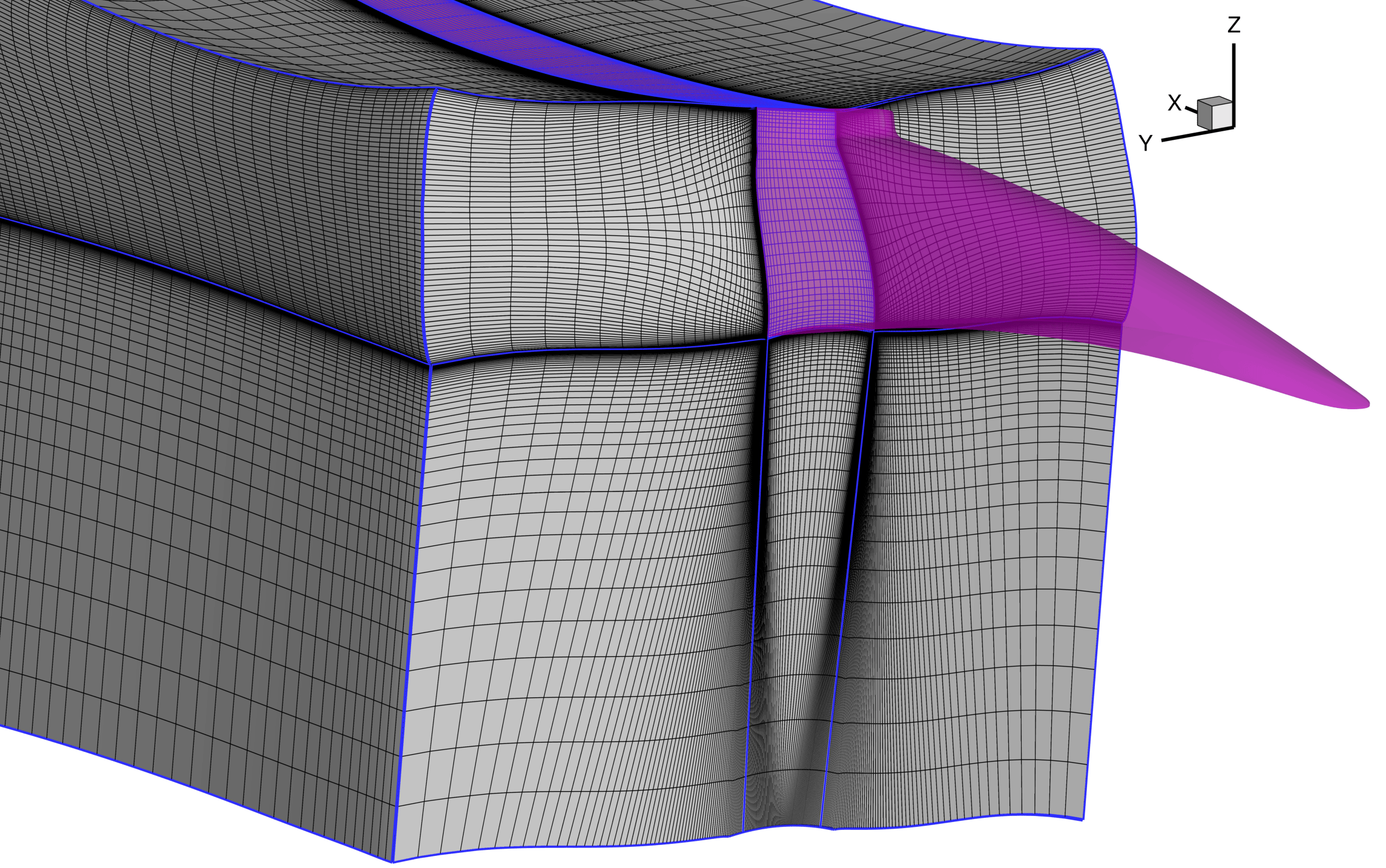
The nose and cusp top grids both follow the same strategy, exemplified below with the nose grids. First, grow outward from the surface. Then split the grid with overlap and extract the L1 surface of the outward volumes, flip, and grow inward.
puts "\tBuilding pylon nose ..."
# --------
GenHypVolGrid PYLON_NOSE.x v.[IBP_nVolP 1] \
              [list \
                  hyptan \
                  specsr \
                  $Par(sr) \
                  $Par(md) \
                  $Par(ds,wall) \
                  $Par(ds,glb) \
                  $Par(klayer) \
              ] \
              [list -5 -5 -5 -5] \
              [list 1.5 150 3]
SplitToNgrids v.[IBP_nVolP 1] v.[IBP_nVolP 3] 2 k 0 7
# --------
IBP_incVol
# --------
ExtractSubs v.[IBP_nVolP 2] v.[IBP_nVol] [list 1  1 -1  1 -1  1 -1]
# --------
IBP_incVol
# --------
ExtractSubs v.[IBP_nVolP 1] v.[IBP_nVol] [list 2  1 -1  1 -1  1 -1]
# --------
IBP_incVol
# --------
ExtractSubs   v.[IBP_nVolN 2] s.[IBP_nSurP 1] [list 1  1 -1  1 -1 1 1]
ReverseInd    s.[IBP_nSurP 1] s.[IBP_nSurP 2] [list revk]
GenHypVolGrid s.[IBP_nSurP 2] v.[IBP_nVol] \
              [list \
                  hyptan \
                  specsr \
                  $Par(sr) \
                  $Par(md) \
                  $Par(ds,wall) \
                  $Par(ds,glb) \
                  $Par(klayer) \
              ] \
              [list -5 -5 -5 -5] \
              [list 1.5 150 3]
# --------
IBP_incVol
# --------
ExtractSubs   v.[IBP_nVolN 2] s.[IBP_nSurP 1] [list 1  1 -1  1 -1 1 1]
ReverseInd    s.[IBP_nSurP 1] s.[IBP_nSurP 2] [list revk]
GenHypVolGrid s.[IBP_nSurP 2] v.[IBP_nVol] \
              [list \
                  hyptan \
                  specsr \
                  $Par(sr) \
                  $Par(md) \
                  $Par(ds,wall) \
                  $Par(ds,glb) \
                  $Par(klayer) \
              ] \
              [list -5 -5 -5 -5] \
              [list 1.5 150 3]
# --------
The final nose and cusp grids are shown below in closeup, with the entire pylon body-fitted immersed set following.
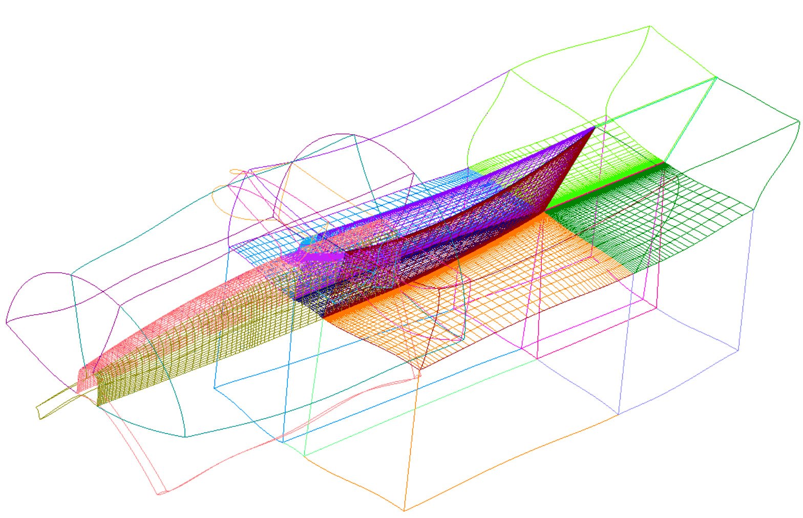
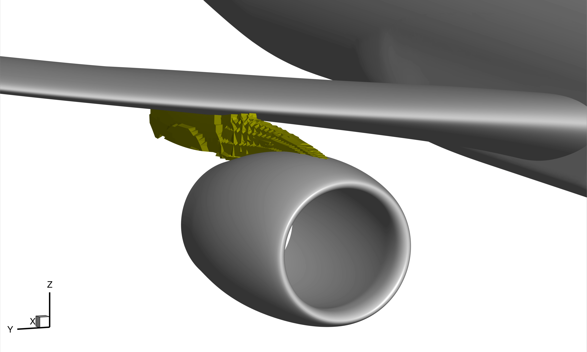
Clearly the body-fitted immersed method takes some setup but with practice it is usually simply making some surface then growing them inward and outward (the block of the aft here was a fancier example), which is MUCH faster than planning and growing weird collar grids. To show the payoff for using this method, see the below comparison of what the pylon would look like if the immersed surface were just tagging the existing grid nodes (left) as opposed to the body-fitted immersed grid nodes (right).
Building And Connecting the Grid
We will be leveraging the power of components, using the same logic as the scripting and connectivity tutorials.
Build the grid by running the run_buildGrid_immBnd.sh script, which calls the
buildProjectGrid_nearBody_immBnd.tcl master grid script to create the
nearBody, then the octFarfield generator to generate the offBody, then
combines the two. Note that the nacelle component has a resolution box placed
around it as part of its component so that we don't have to use a different
nearBody surface triangulation for the offbody generation. Additionally, this
copies over any immersed boundaries, which should be modified in the scripts as
needed when copied over to account for parameters like pitch, etc. The naming
convention is usually immGeom_COMPNAME_SUBNAME.i.tri.
To run connectivity, follow the instructions in the connectivity tutorial,
keeping in mind that you must use the init_connectivity_immBnd.sh script
instead of init_connectivity.sh. Running connectivity locally with 55 threads
takes roughly 10.6 seconds and has 0 orphans.
B2BExtractor :
  extractB2Bs  : true
  onlyFullB2Bs : true

...

immersedBoundaries:
  -
    fileName : immGeom_PYLON.i.tri
    fileType : tri
    bcname :   pylon

...

 bc :
   -
     names :    [pylon]
     type :     BCWallViscous
     location : offBody
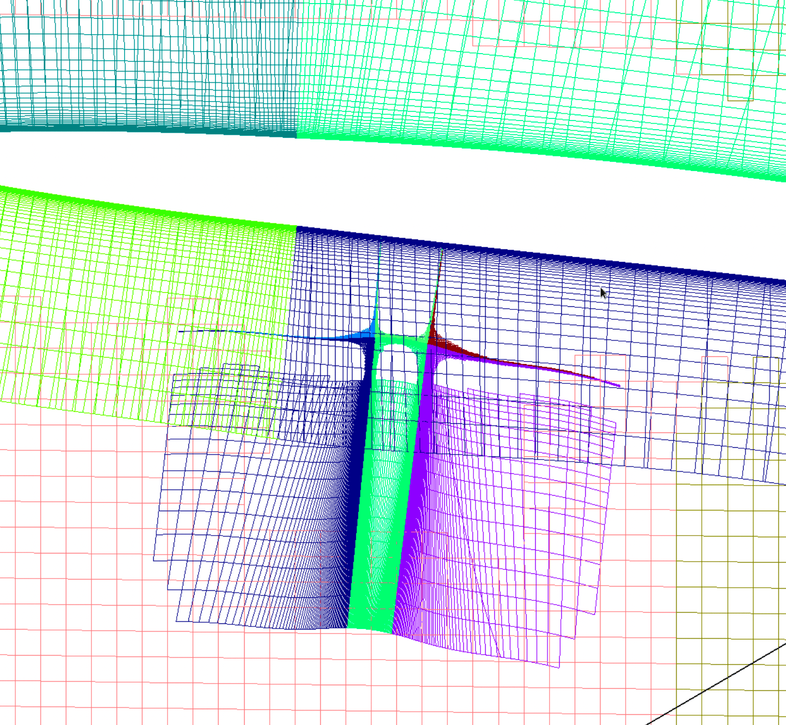
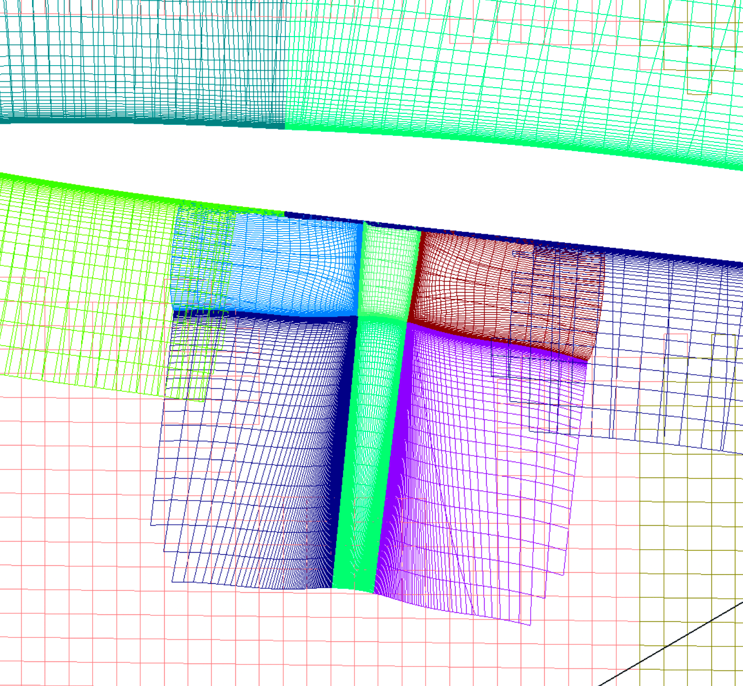
Priorities become significant when adding new components to an existing system. We want the newly added body-fitted immersed grids to be kept so that the immersed geometry is well represented (it's why they're there in the first place). However, we see below on the left that simply adding them in naively causes them to be mostly removed. This is because the existing nearBody grids have a priority of at least 100. To keep them and obtain the grid optimization on the right, the priorities are updated as seen below.
overset :
  zoneSpecific:
   -
     # All non-nose or collar near-body zones.
     zones :    [1, 9-22, 29-40]
     priority : 100.0
   -
     # Non-aft-top pylon zones.
     zones :    [42-47, 54-61]
     priority : 200.0
   -
     # Nacelle resolution zones.
     zones :    [41]
     priority : 400.0
   -
     # All nose and collar near-body zones.
     zones :    [2, 3-8, 23-28]
     priority : 1000.0
   -
     # Pylon aft top zones.
     zones :    [48-53]
     priority : 1.0e+10
It is also important to note that while it is possible to allow immersed grids
to intersect with wall geometry, this is not the strategy employed here.
Immersed-wall component intersection is being looked into as a design feature,
and employs an immersed method which is more of a boundary condition than a
simple penalty term. In such a situation, the zones pertaining to the immersed
boundary can be stated within the immersed entry as zones during connectivity
and the solution, and they would become immersed inside the wall geometry
instead of blanked, with a special correction applied during solution. This
feature has not been extensively tested and is still experimental. Here, we
don't care if minor pylon shape errors exist very close to the intersecting
boundaries with the wing and nacelle, and so we blank any immersed grids inside
those wall shapes, but set the priorities such that they are retained very
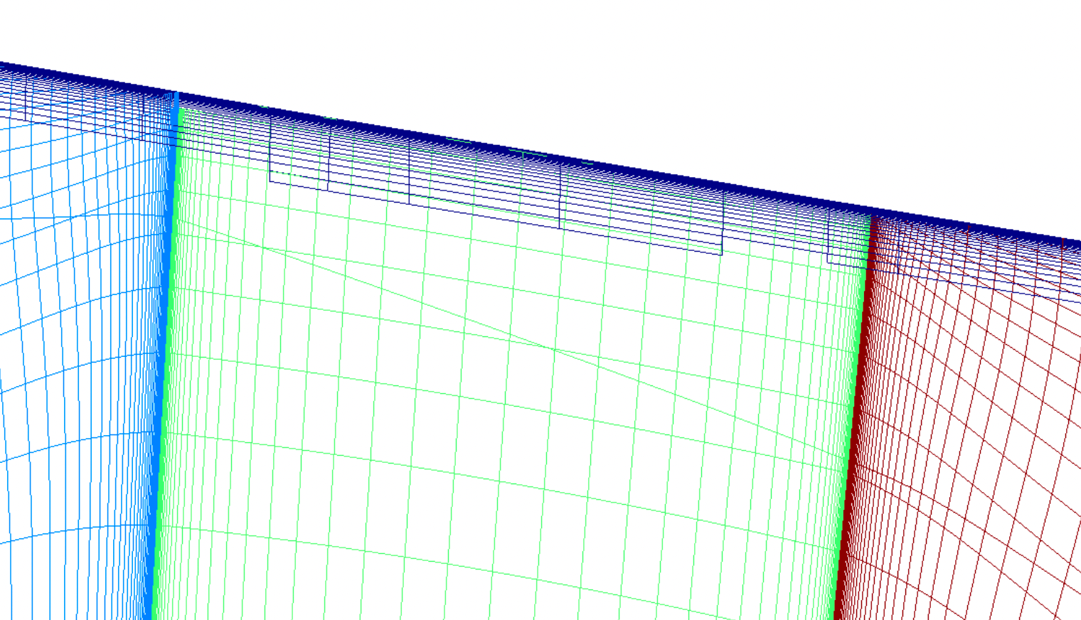
close to the walls. Below is a picture of the grids near the wing-pylon
intersection.
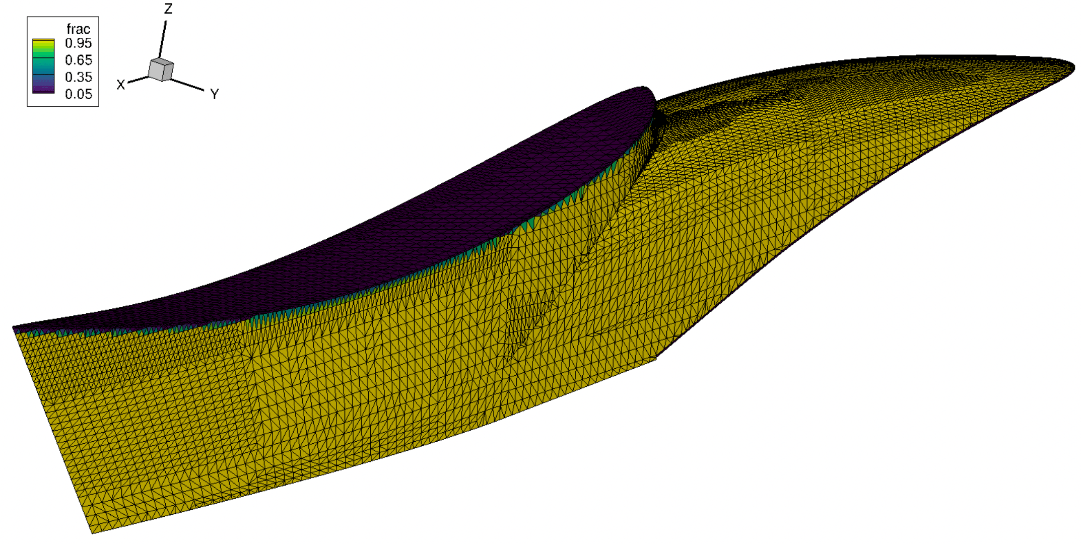
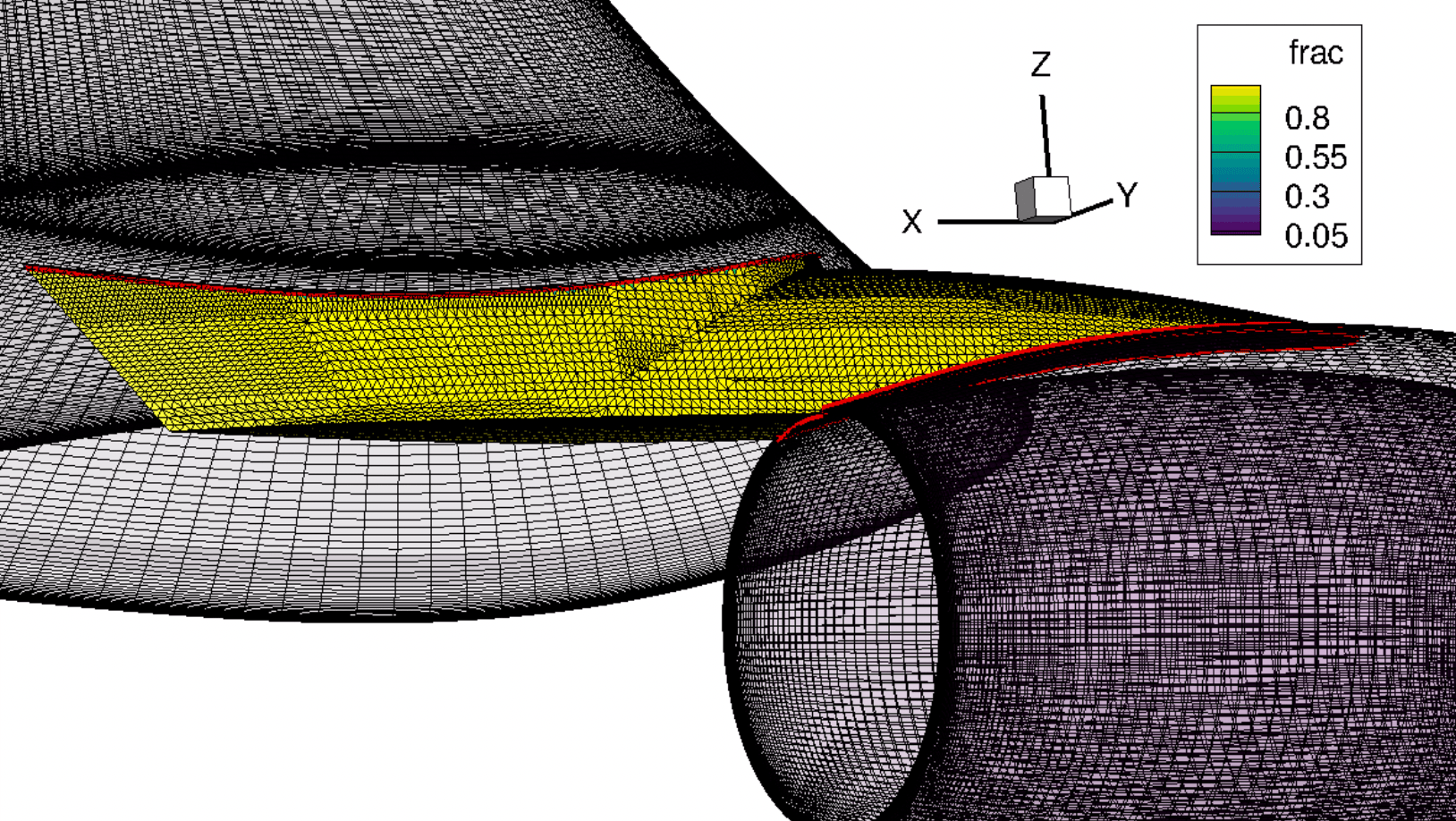
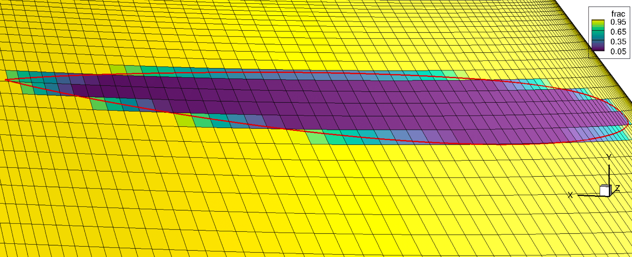
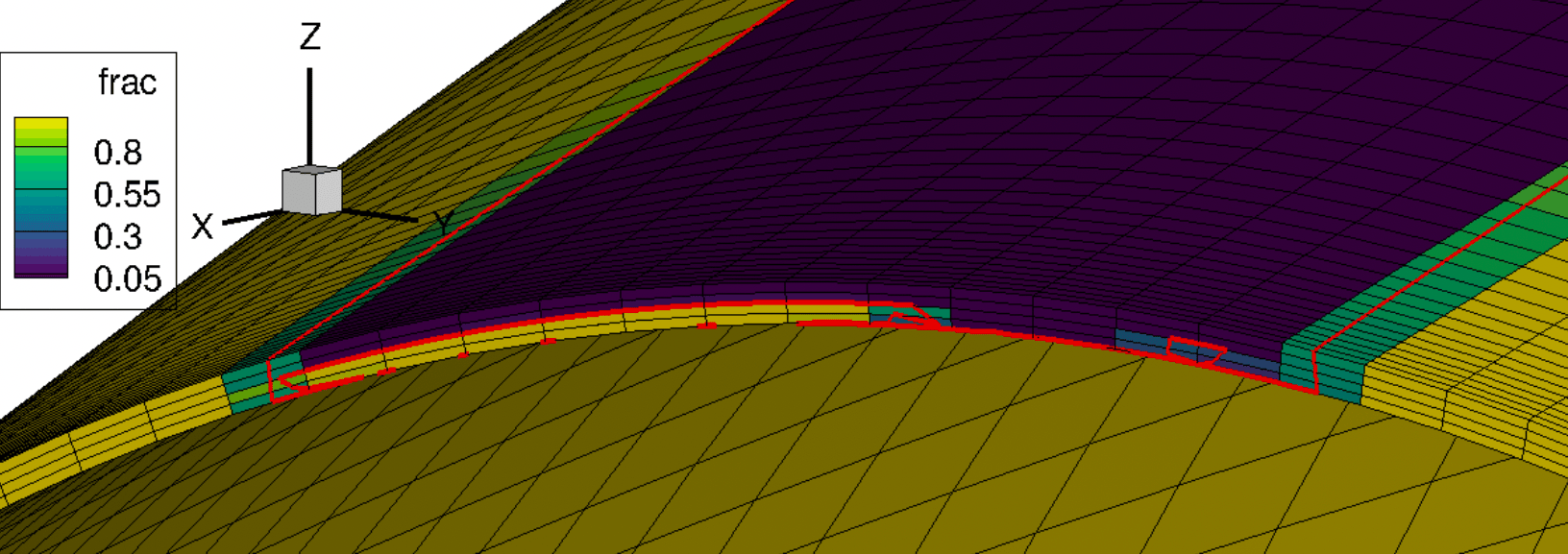
The overlapper utility run after the connectivity process creates panel weights on both the walls and the immersed boundaries, and accounts for intersections between the two, as seen below in which the red lines are the intersection curves.
Running the Solver
The steps for running the solver are effectively the same as the RANS
tutorial, tutorial, but the 'init_RANS_immBnd.sh' script
is used instead of init_RANS.sh, and you plan to run on NAS you need to
additionally push any immGeom_* files (in this case just
immGeom_PYLON.i.tri) there if you weren't building the grid on NAS.
The LAVA_solver_RANS_immBnd.yaml input file has the following additions to
its LAVA_solver_RANS.yaml sibling, shown below.
immersedBoundaries:
  -
    fileName :              ../immGeom_PYLON.i.tri
    fileType :              tri
    bcname :                pylon
    updatetype :            drivetozero
    interpOffsetDist :      4.875e-05
    timescale :             1.0e-3
    timescalevaluestype :   specified
    timescaleintervaltype : iter
    timescaleramptype :     discrete
    timescaleinterval :     [100, 200, 300, 400]
    timescalevalues :       [1.0e-4, 1.0e-5, 1.0e-6, 1.0e-7]

...

bc :
  -
    names : [fuse, wing, tail, nacelle]
    type :  BCWallViscous
  -
    names :     [pylon]
    type :      BCWallViscous
    wallmodel : saLaw
The immersed pylon is placed in its own BC with a wall model. When calculating surface variables, it will interpolate from the solution according to the wall model law (sa in this case). Note that at intersections with other components, the cell center of intersected elements could be within the intersected body, thus making interpolation from the solution incorrect. During the overlapper panel-weight generation, interpolation locations for intersected immersed triangles are moved to guaranteed wetted locations to account for this possible inaccuracy.
The immersedBoundaries yaml sub-dict can have different entries for each
immersed surface you have defined. In this case its just the pylon. Each entry
is linked to the appropriate BC name. The interpOffsetDist is the wall-model
interpolation distance off the wetted cell center for load calculations. The
timescale settings have to do with how the momentum penalty is applied. The
smaller the timescaleValues, the more of a penalty is applied: we have found
that 1e-7 or 1e-8 is usually required to impose a wall-like effect on the flow.
The update type is how the immersed penalty is applied. Here we are pushing the
momentum to zero within the immersed region rather than hard-setting it (which
tends to be unstable). The values of the timescale also ramp over a series of
intervals, as starting out with the most aggressive momentum penalty can be
numerically unstable. Here, the final timescale is applied after timestep 400.
Upon submitting the solver, the following warning pops up:
--------------------------------------------------------------------------------------------------------------------------------------------
Warning msg on proc(0) : Could not find one or more donor cells for IB Cells and/or their offsets - writing to IBSurf_elemFailedInterps.plt.
--------------------------------------------------------------------------------------------------------------------------------------------
This means that some of the immersed surface elements with non-zero panel
weights couldn't find legal computational cells to interpolate their wall model
values from. Let's investigate why this is the case. Alter the
LAVA_solver_RANS.yaml file in your solution subdirectory by adding the
following entries to the curvsolver and overlapper sub-dictionaries:
curvsolver:
  writeIBWallModelInterpNodes : true
  overwriteIntegrationWeights : true

overlapper:
  writeIntersections : true
This will force the solver to re-calculate the panel weights with the overlapper utility. The following files will be written in the overlapper directory:
overlap_wallElemFracs.plt: wall panel weights in a viewable format.overlap_IBElemFracs.plt: immersed panel weights in a viewable format.overlap_isects_final.dat: the intersection curves between immersed and wall geometry.IBSurf_matchLocVecs.dat: The vectors of wall model interpolation from immersed surface elements.
If we re-run the solver and open these files (along with the
IBSurf_elemFailedInterps.plt file written in the solution directory) we can
perform the following assessment. The left and right figures below show the
intersections of the pylon with the wing and nacelle, respectively. Panel
weight fractions are shown on the immersed surface, the intersection curves are
show in red, and the immersed wall model interpolation vectors are shown in
teal for elements which have non-zero integrable area. Note how the
interpolation vectors have been repositioned to a fluid location if the cell
has been intersected.
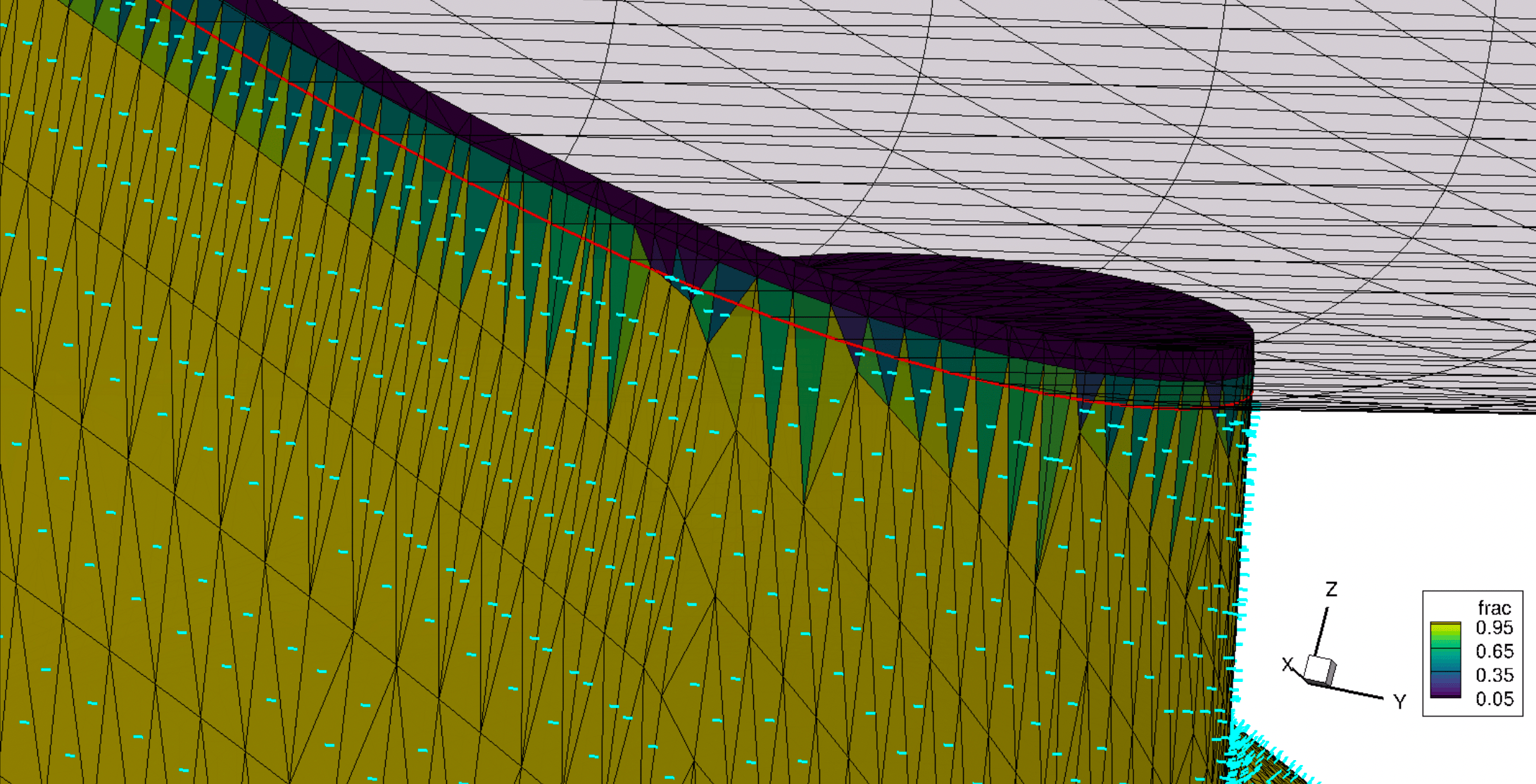
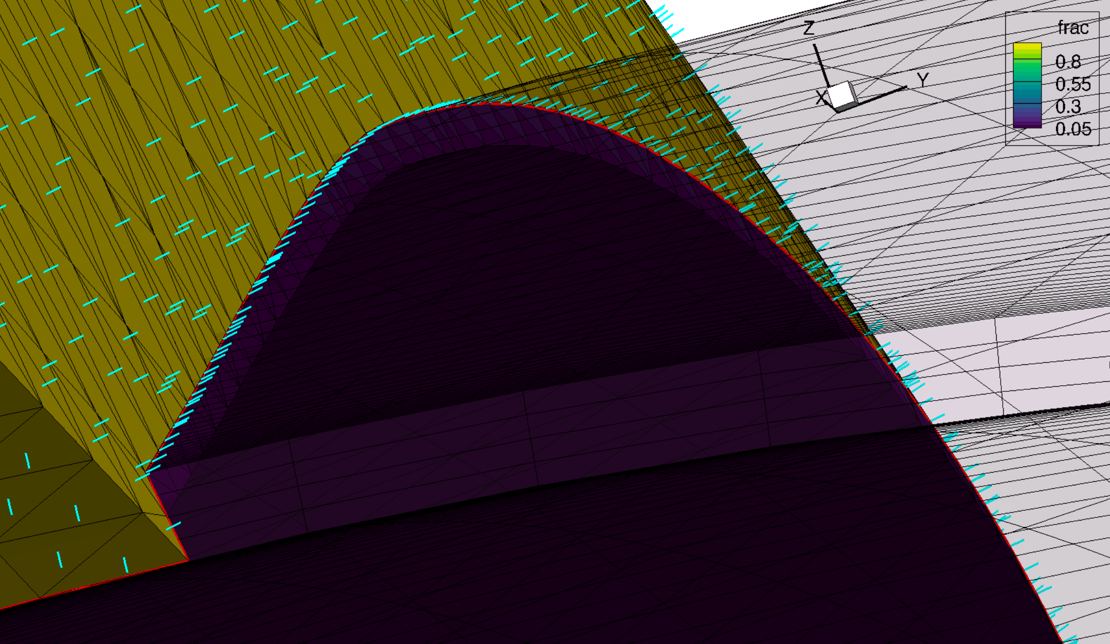
The intersection with the wing is properly (normally-ish) intersecting, through generally-orientated tri-elements. The intersection with the nacelle is along a feature curve of the triangulated surface (the triangles respect that surface), and so the intersections with the nacelle is along many triangle edges: thus the clustering of interpolation vectors near the nacelle surface. The pylon geometry intersects the nacelle properly along its length, but note how at the trailing edge the pylon geometry abuts the nacelle and is more parallel than intersecting.
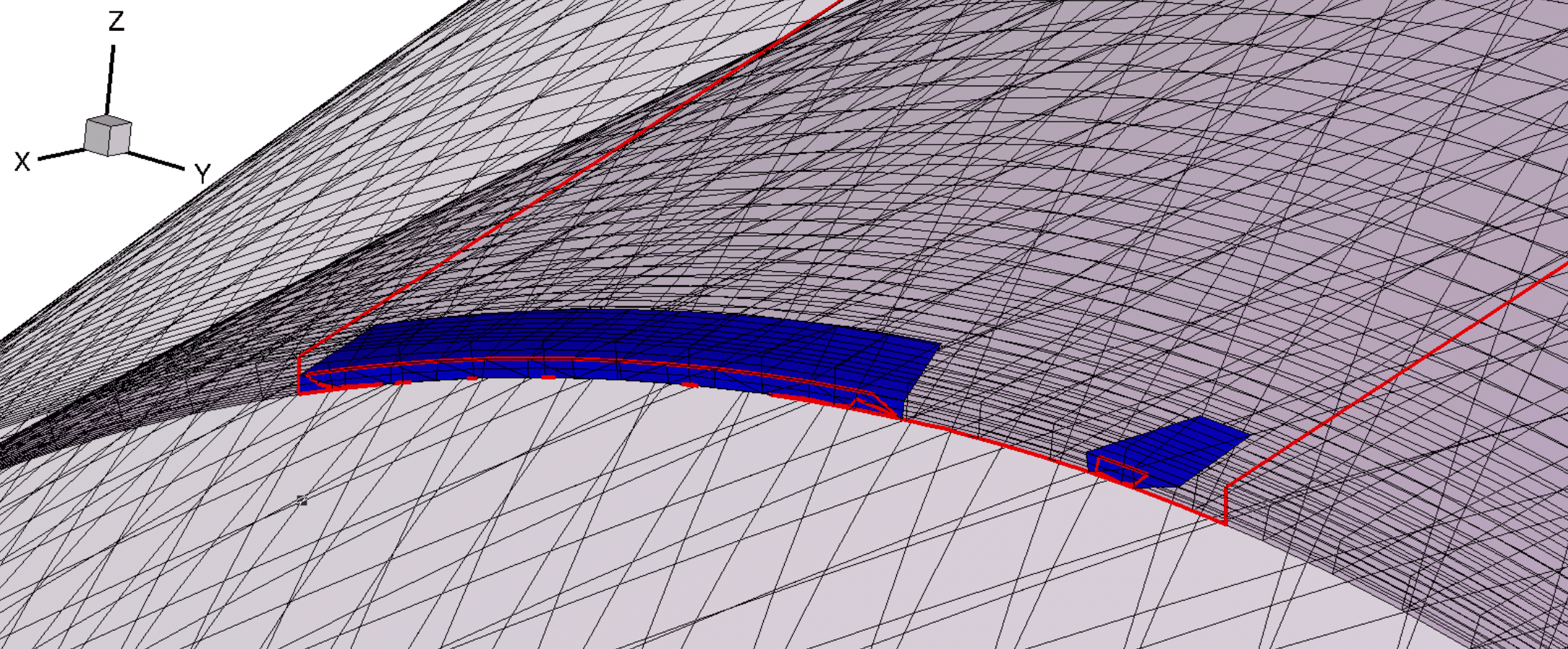
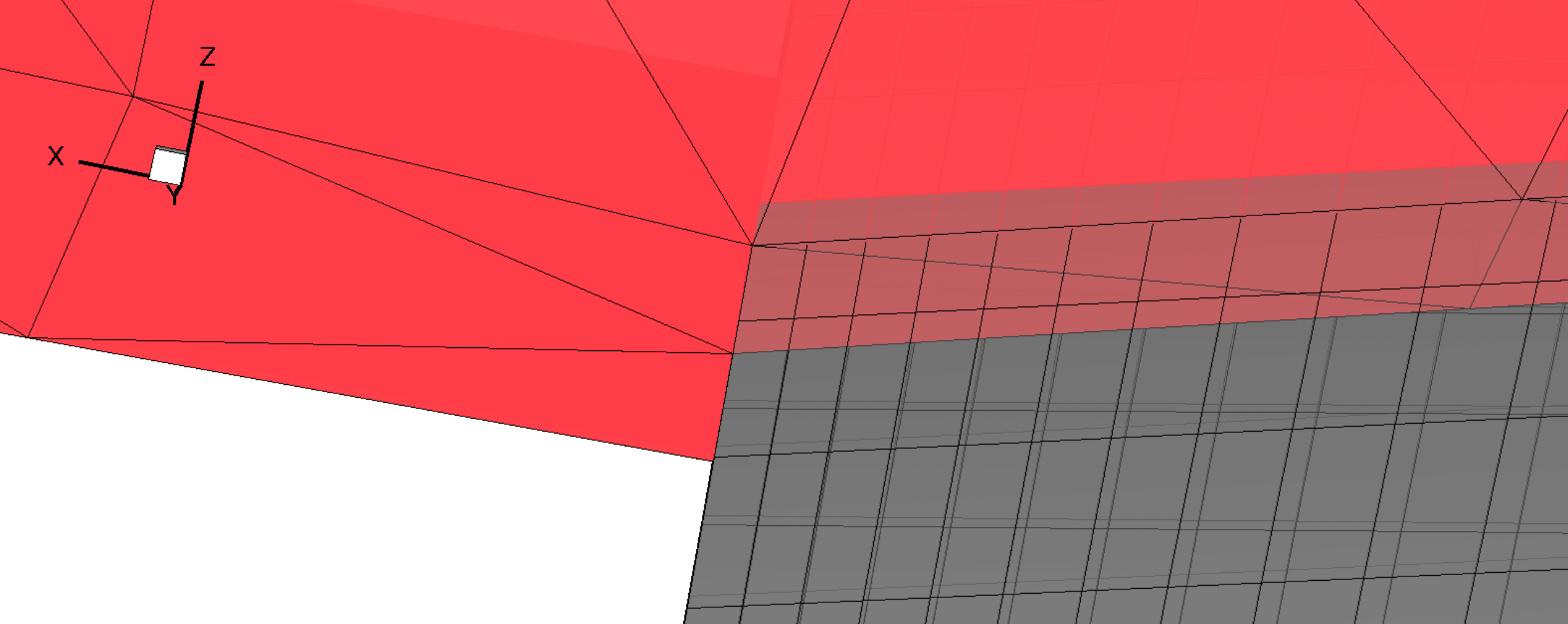
The immersed elements which failed to find legal interpolations are shown below on the left. Note how they are all on the nacelle trailing edge. The intersection curves are shown in red and at the trailing edge we see that the parallel alignment has caused spurious intersections to have been found due to tolerance issues. Any integrable surface element which understands it intersects with another component will have a non-zero fraction and will attempt to find elements from which to interpolate field values. In this case, the 'intersecting' (abutting) geometry has normals pointing in different directions, and so any interpolation vectors from their elements will look inside the intersected geometry - thus the error. This is shown more clearly in the left figure below, in which the pylon geometry is red and the nacelle is grey. 'Parallel' geometry intersection tolerance uncertainty is a known issue which will be addressed at some point in the future, but is not an issue if you ensure your immersed geometries properly intersect the relevant wall geometry.
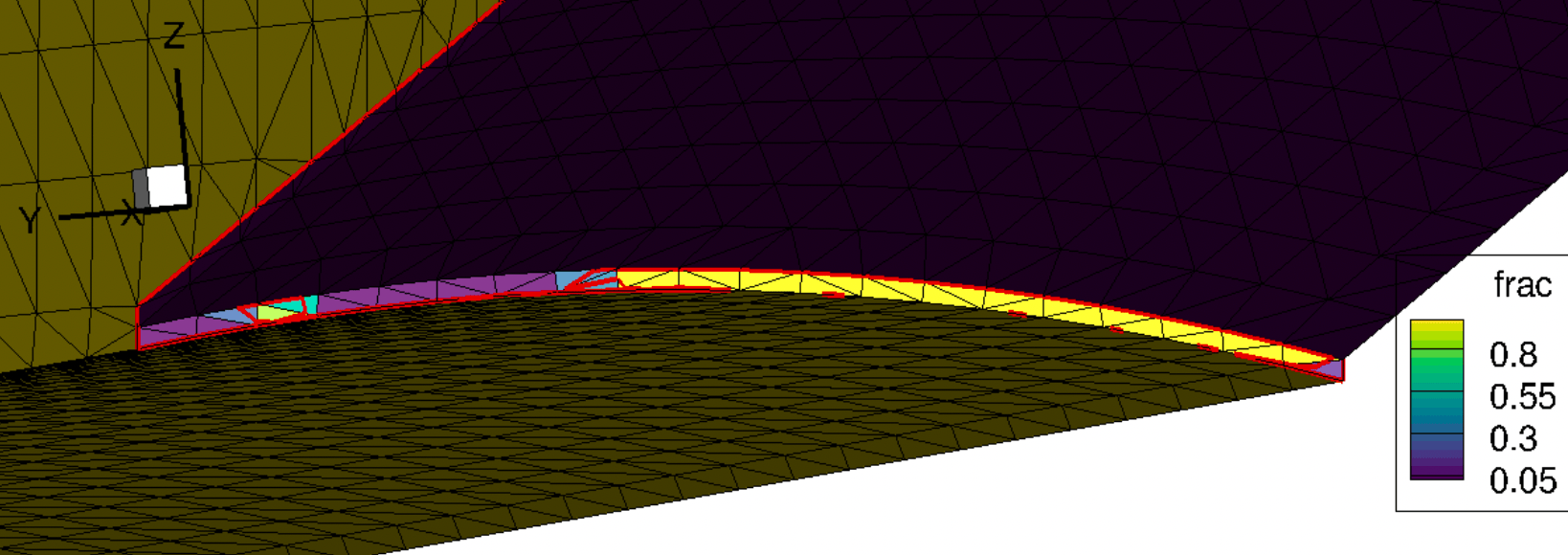
Here, these interpolation problem cells are not an issue because while their panel weights are non-zero at portions of the abutting geometry (as below - pylon left and nacelle right), the geometry should technically be non-integrable and the solver will set their integration fractions to 0 at runtime if no integration location can be found.
Solution Assessment
You can assess this solution convergence using the same interrogations performed in the RANS tutorial.
The videos below show a sweep of the converged solution's Mach and eddy viscosity ratio along the pylon, with roll-up occurring along its length indicative of the viscous and inviscid effects the pylon has on the flow within the pressurized region underneath the wing.