Conducting a Grid Refinement Study
Creating a set of grids for a convergence study is standard procedure to bound a grid's truncation error. Possible options within the context of the LAVA project file system are:
- Incorporate the refinement factors within the grid growth scripts. This
requires the grid parameters in
parm/MakeParm.tclto be dependent on grid level (already inherent), and for a set of starting surface grids to exist within each component's geom sub-directory. Likely, conditional grid growth arguments such as splay have to be implemented iteratively in the components' tcl scripts in order for the now denser grids to have proper overlap, non-folded elements, etc. - Build a new volume grid from scratch using EPOGS for each refinement level desired with appropriate refinement of grid metrics. This may result in needing to manually correct individual grids for each level (see the EPOGS tutorial for a brief discussion on this).
- Use LAVA's
refineutility to take existing volumes and refine them by a factor. If refinement issues arise, the growth parameters of the level one grids (i.e. the starting grids) must be adjusted to allow for a well-posed starting point. This generally doesn't require much effort.
We chose to adopt the last option for this tutorial. As show in the figure below, LAVA's refine executable takes each block and directionally parameterizes each block curve with a spline, redistributes it with a refined point set in parameter space, and then maps that redistribution back to physical space.
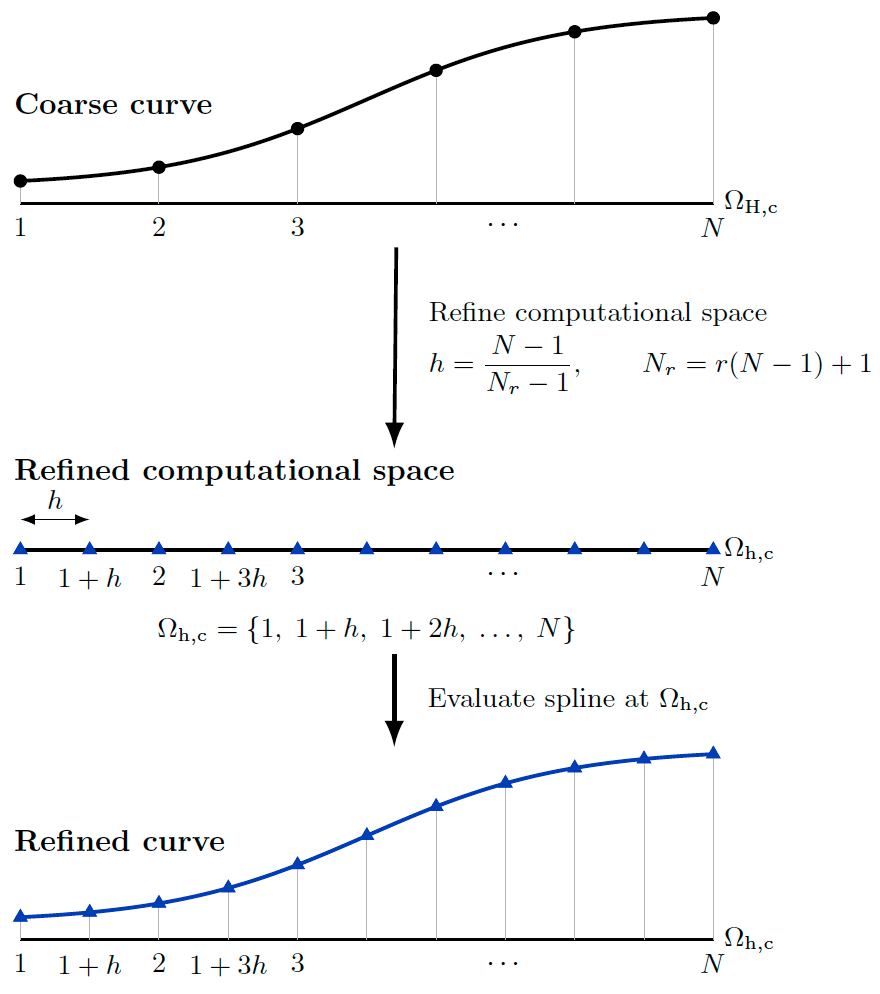
There is currently no projection back to CAD, so one caveat is if significant c1-discontinuity or repeated alternations between concavity and convexity exists within the parameterized curve curvature then the refined curves may no longer well-represent the true model geometry (this is no worse than refining grids using existing CGT functionality such as SrapRedist). For this reason the surface grids were built a-priori to delineate feature lines that should be respected.
Building the Refined Grid Set
To run the refinement procedure first navigate to the desired run sub-folder
(pick the one you created for the scripting
tutorial). If you do not have the grid.x and
grid.bc files required as a starting point for this tutorial, either do the
project grid scripting tutorial or download
them from that tutorial. Once those files exist, run the run_refineGrid.sh
script, shown below, making sure the GROUP_ID, LAVA_EXE_DIR, and
LAVA_EXE_SUFFIX, and OMP_NUM_THREADS variables are set in envVars.sh.
# Define a number of refinements (1.414214 and 2.0 here), then
# perform the refinements in appropriate sub directory.
# Use sed to alter the yaml files to have the right refinement factor.
# This script assumes that we will be performing a RANS convergence study,
# and so also copies in and appropriately alters the files needed to run
# a RANS solution on NAS.
# ---------------------------------------------------------------------------- #
factOnes=(1      2)
factDecs=(414214 0)

baseDir=$( cd -- "$( dirname -- "${BASH_SOURCE[0]}" )" &> /dev/null && pwd )

source $baseDir/envVars.sh

mkdir -p soln_RANS

cp $baseDir/auxFiles/LAVA_solver_RANS.yaml       ./soln_RANS/
cp $baseDir/auxFiles/LAVA_solver_RANS_athena.pbs ./soln_RANS/

sed -i "/#PBS -W/c\\#PBS -W group_list=$GROUP_ID" \
       LAVA_solver_RANS_athena.pbs

for ((factI=0; factI<${#factOnes[@]}; factI++)); do

    # Make and enter refined grid folder.
    # ------------------------------------------------------------------------ #
    refFolder="refinedGrid_factor${factOnes[$factI]}p${factDecs[$factI]}"

    mkdir -p $refFolder
    cd       $refFolder
    # ------------------------------------------------------------------------ #

    # Refine the grid.
    # ------------------------------------------------------------------------ #
    cp ../grid.bc .
    cp $baseDir/auxFiles/LAVA_refine.yaml .

    sed -i "/  factor : 1.0/c\  factor : ${factOnes[$factI]}.${factDecs[$factI]}" \
           LAVA_refine.yaml

    $LAVA_EXE_DIR/refine.$LAVA_EXE_SUFFIX LAVA_refine.yaml

    mv surface.x grid.sur
    rm LAVA_refine.yaml
    # ------------------------------------------------------------------------ #

    # Get and update the files needed to run RANS on NAS.
    # ------------------------------------------------------------------------ #
    jobName="LAVA_solver_OGSCRM_AOA2p5_L${factOnes[$factI]}p${factDecs[$factI]}"
    factor="${factOnes[$factI]}.${factDecs[$factI]}"
    nNode=$(echo "(($factor * $factor * $factor) + 0.5) / 1" | bc)

    mkdir -p soln_RANS

    cp $baseDir/auxFiles/LAVA_solver_RANS.yaml       ./soln_RANS/
    cp $baseDir/auxFiles/LAVA_solver_RANS_athena.pbs ./soln_RANS/

    sed -i "/#PBS -l select/c\\#PBS -l select=$nNode:ncpus=256:mpiprocs=4:model=tur_ath" \
           soln_RANS/LAVA_solver_RANS_athena.pbs
    sed -i "/#PBS -N/c\\#PBS -N $jobName" \
           soln_RANS/LAVA_solver_RANS_athena.pbs
    sed -i "/#PBS -W/c\\#PBS -W group_list=$GROUP_ID" \
           soln_RANS/LAVA_solver_RANS_athena.pbs
    # ------------------------------------------------------------------------ #

    # Back to base grid folder.
    # ------------------------------------------------------------------------ #
    cd ..
    # ------------------------------------------------------------------------ #
done
# ---------------------------------------------------------------------------- #
For each grid level defined with a ones and decimals place, a level-named sub-folder is created and the refine executable is called within it to create a local grid. The grid within these sub-folders is named the same as the base grid level so that other run scripts can be called on them (e.g. connectivity - see below). The BC file is copied in because the BCs shouldn't have changed. In this case we are creating grids that are a factor of 1.414214 and 2.0 denser than the original.
The input file to the refinement utility is shown below. Note how the grid to
be refined is one level up from the sub-directory we have created. When it is
imported by run_refineGrid.sh, the factor entry is modified appropriately.
The surface grid is the portion of the refined grid defined by the bc file.
Note that if partial BCs existed (the ranges were not [1,-1]) then the bc file
would have to be altered prior to refine being called to ensure accurate
surface extraction.
refine:
  factor : 1.0
  coarseGridFile : ../grid.x
  refineGridFile : grid.x
  nSmooth : 0
  writerecordmarkersingrids: false

surface :
  extract : True
  surfaceGridFile : surface.x
  bcFile : grid.bc
  surfaceBCNames : [fuse,wing,tail]
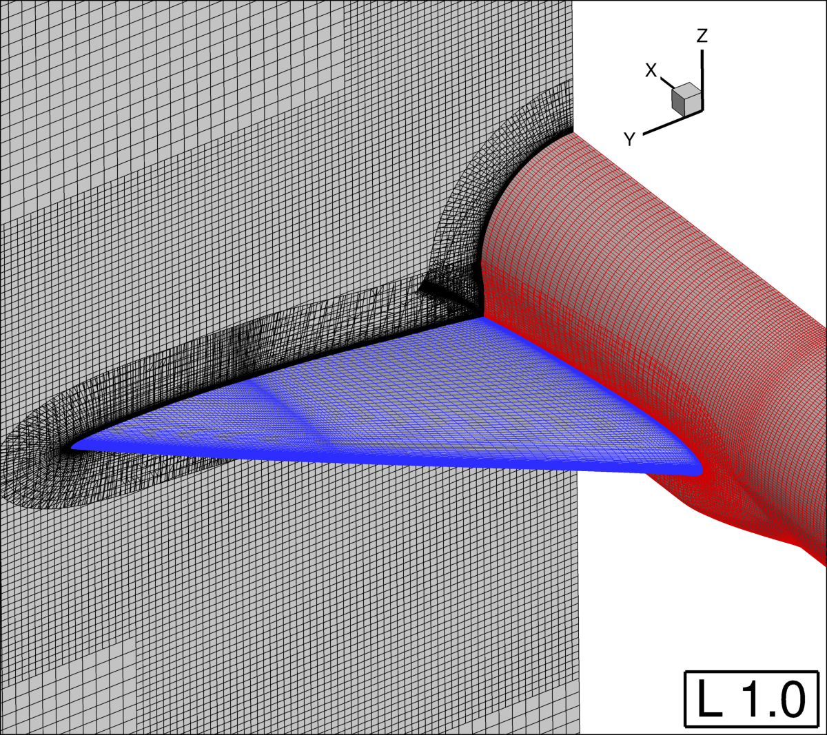
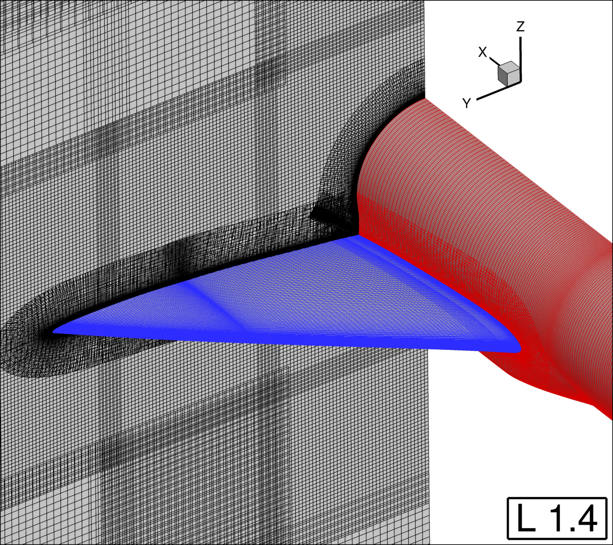
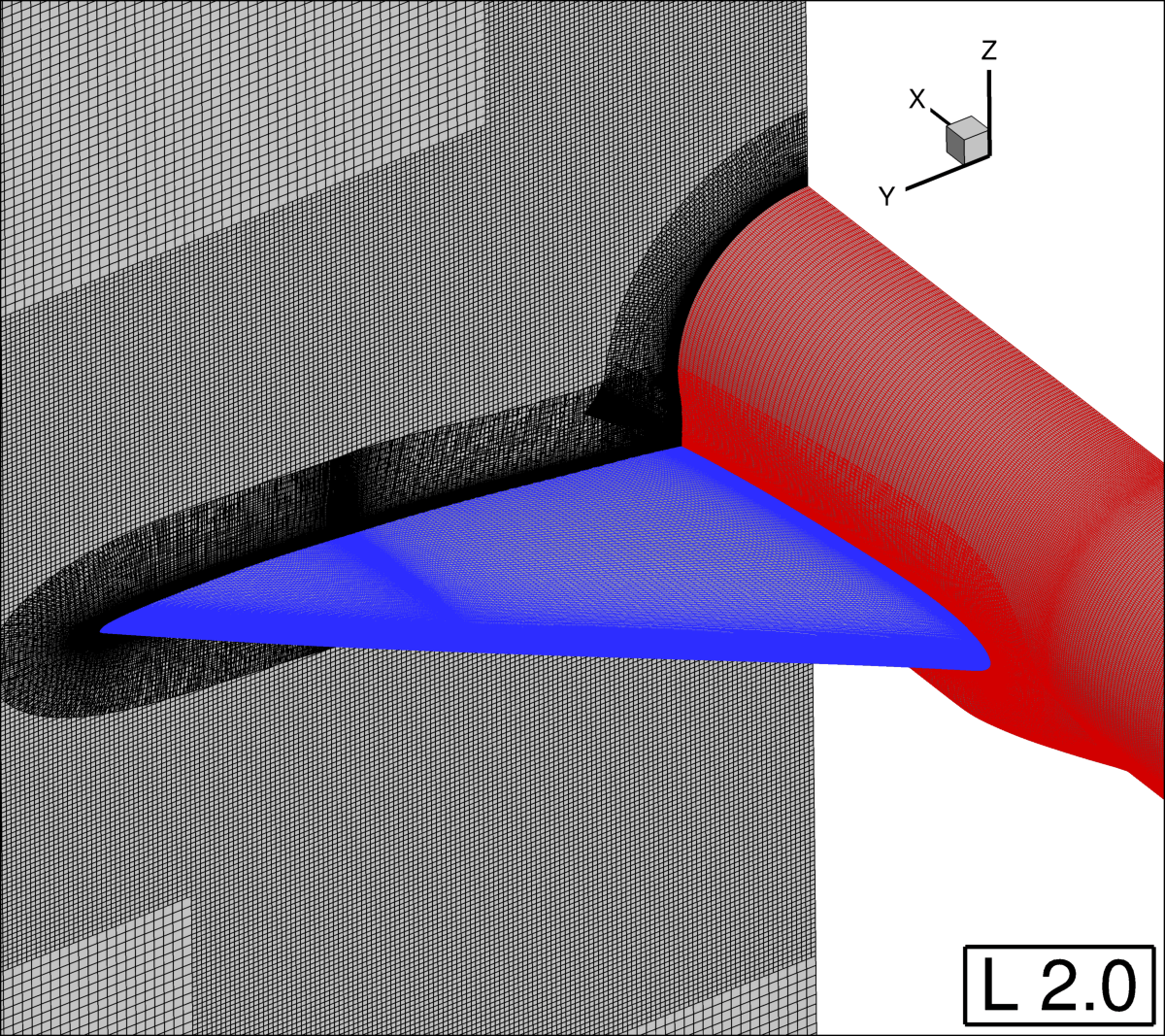
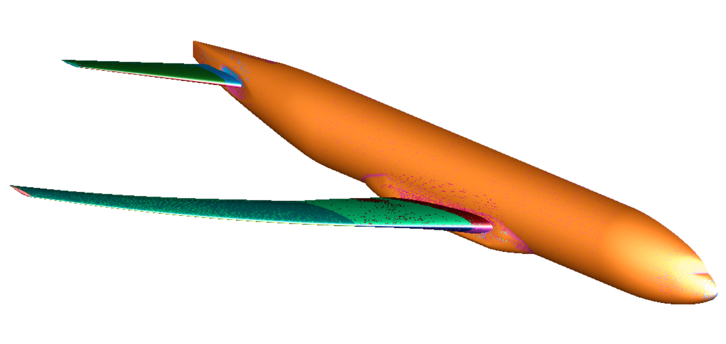
Slices and surfaces of the refined grid set can be seen below. The entire grid system has been refined, but note that there are options to refine individual grids to different levels, or directionally.
Connecting and Assessing the Refined Grids
Run the run_connectivity.sh script within each refined grid folder
(refinedGrid_1p414214, refinedGrid_2p0), or run on NAS as described in the
connectivity tutorial: no changes need
to be made to the connectivity files themselves because the grid files are
named as expected. The level 1.414214 grid takes 12 seconds with 56 threads to
run the connectivity script and has ~68 million nodes, while the level 2.0 grid
takes 30 seconds and has ~189 million.
There are generally three things to check for issues on a refined grid:
- Negative Jacobians: Open the
grid.x.ihcfile inovergridand click DIAGNOSE and then the show box next to Jacobian in the bottom right. If any of the table entries have non-zero count then view them in the grid. Look at your level zero grids in the same locations (likely they will be almost folded in the now problem areas) and alter the grid scripts to smooth or splay them more to prevent refinement issues, then rerun refinement. - Orphans: It is unlikely that orphans will appear due to overlap issues
that didn't already exist in the starting grid because the overlapped region
isn't reduced. However, the shape of the geometry surface may have slightly
changed if the spline across a large portion of a body which, for instance,
undulates. More laxity in projection may be needed. Clicking DIAGNOSE within
overgridand then All under orphan analysis in the mid right will count and highlight orphans. - Commensurate B2Bs: The connectivity process assesses and writes a new B2B file. One indication of refinement going wrong is if the B2B file created doesn't match that of the starting grid. Diff the two to double-check.
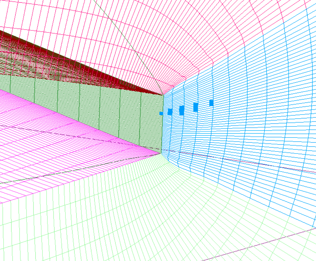
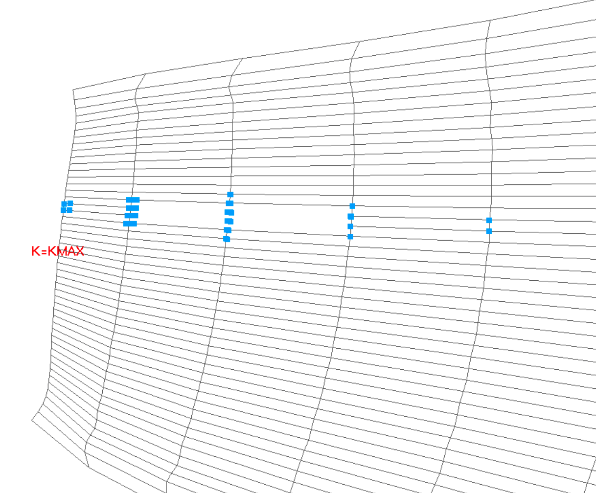
The level 1.414214 grid does not show any issues for these checks. The Level 2.0 however, shows the orphans on zone 5: the inboard wing trailing edge. Zooming in and cycling through constant L of grid 5 shows that the orphans surround a hole that has been created in grid 5 from [J 17->18, K 47, L 8->9]:
These kind of localized 'hash' patterns of orphans generally mean an edge or
two has been cut, but we will re-run connectivity with a debug node to be sure.
Alter the LAVA_connectivity.yaml file to have the following additional
debugNode entry. The run_connectivity.sh script is designed so that
alterations to the yaml file will not be overwritten.
When connectivity is re-run now, we see output with a 'Debug Node' prefix. Assessing the output from debug nodes can be complex and the manual exists in part to make this output less opaque. We focus in on the following lines, which state that the portion of block 1 (the fuse) which intersects one of the edges of this node is too far away to project to given the relative size of the elements, which means connectivity doesn't think they are the 'same' surface.
[[Debug Node (Blk,j,k,l)                5   17   47    8]] (thread    27): Checking edge [   17   47    8] to [   17   47    9] for surface intersection ...
[[Debug Node (Blk,j,k,l)                5   17   47    8]] (thread    27):     Start node closest surfNode Blk/i/j/k:     5   17   47    1
[[Debug Node (Blk,j,k,l)                5   17   47    8]] (thread    27):     End node closest surfNode Blk/i/j/k:     5   17   47    1
[[Debug Node (Blk,j,k,l)                5   17   47    8]] (thread    27):     Considering intersection     1 of     1 with block     1...
[[Debug Node (Blk,j,k,l)                5   17   47    8]] (thread    27):         Found surface relation between intersected face  114099 and edge start node.
[[Debug Node (Blk,j,k,l)                5   17   47    8]] (thread    27):         Edge start node dist from wall node to cut node:   0.00001302
[[Debug Node (Blk,j,k,l)                5   17   47    8]] (thread    27):         Edge start node max local deviation offset lim:   0.00000378
[[Debug Node (Blk,j,k,l)                5   17   47    8]] (thread    27):         Start dist from wall outside of surface deviation limit: cut edge.
[[Debug Node (Blk,j,k,l)                5   17   47    8]] (thread    27):         At least one edge is linked to the block surface: checking unrelated interpolated intersection overlap ...
[[Debug Node (Blk,j,k,l)                5   17   47    8]] (thread    27):         Edge node dist from interpolated wall node to cut node:   4.05455871
[[Debug Node (Blk,j,k,l)                5   17   47    8]] (thread    27):         Edge average node max local deviation offset lim:   0.00000378
[[Debug Node (Blk,j,k,l)                5   17   47    8]] (thread    27):         Interpolated intersection is also outside of surface deviation limit: cut edge.
[[Debug Node (Blk,j,k,l)                5   17   47    8]] (thread    27):     Intersected     1 times with surface projs, at least one of which can't be treated as the same surface: blanking both edge nodes.
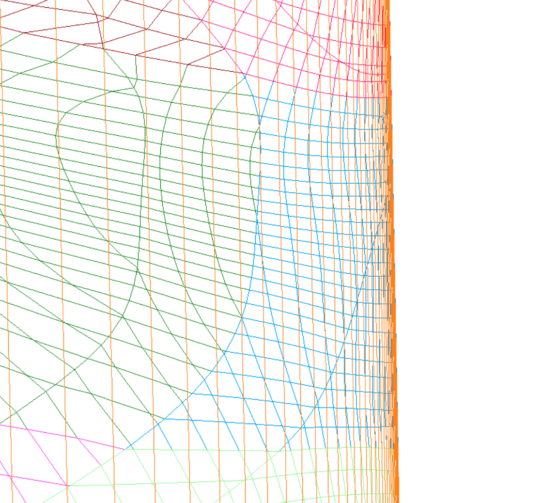
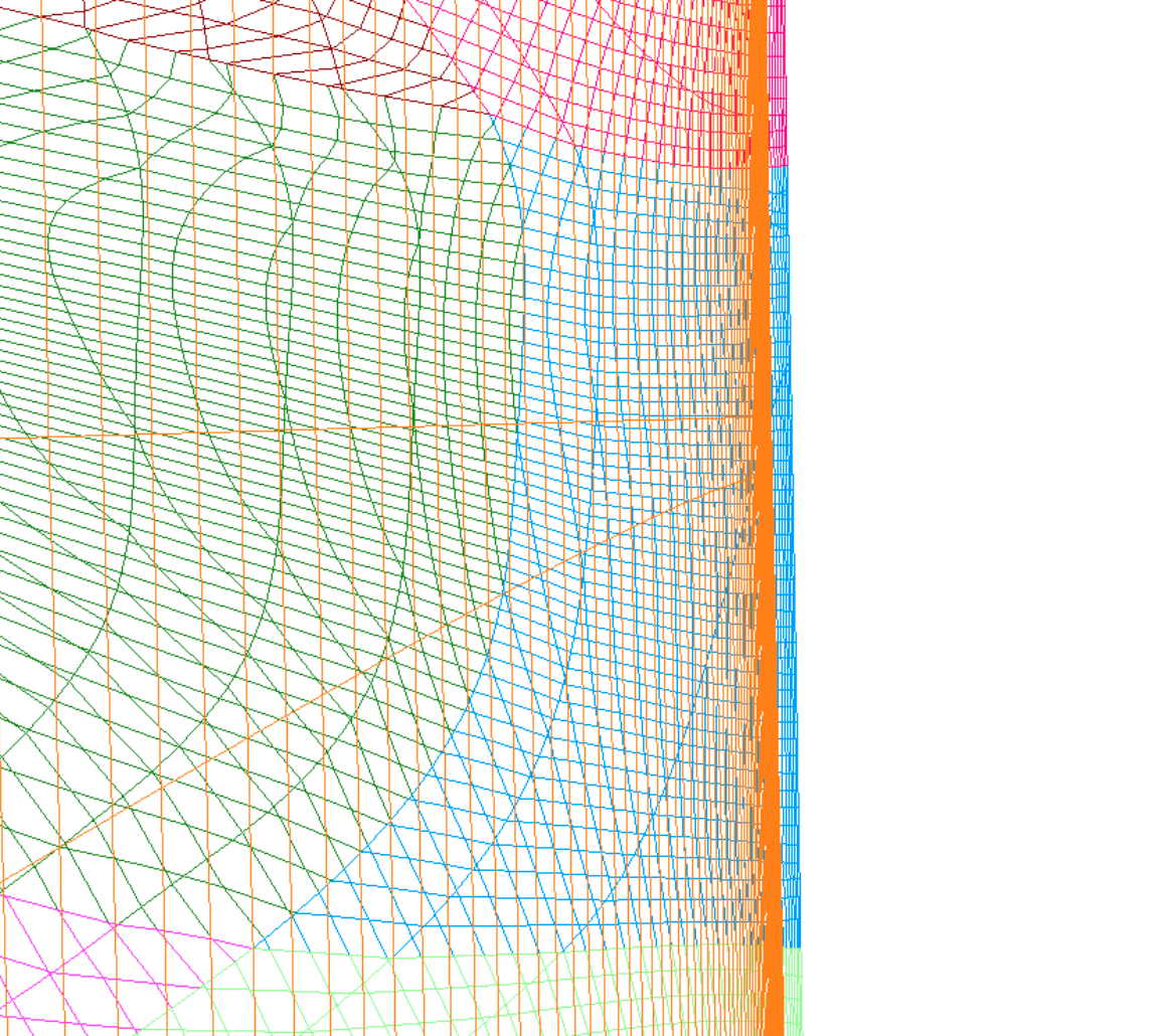
Taking an x location near the orphans (4.053641), we take a slice of the un-cut grid.x file and zoom into trailing edge intersection with the fuse to find that there is indeed a slightly larger offset of the fuse on the refined grid (right) than was on the original grid (left):
Opening both the original and refined grid.sur files with the Flat Shaded Display Option checked shows that splining the long fuse undulations has caused some minor differences in the fuse which are mostly irrelevant except for this problem location:
The fix for this issue is simple: slightly increase the distance surfaces on
block 5 are allowed to accept projection onto other surfaces. This is done
through the edgeFactor option (defaulted to 1) assigned to block 5 through a
zoneSpecific option by adding the following lines to the
LAVA_connectivity.yaml file and re-running run_connectivity.sh:
overset :
  zoneSpecific:
   -
     # Allow block 5 to project just a bit further (onto block 1).
     zones :      [5]
     edgeFactor : 1.2
One could also argue that the fuselage component should be split into smaller
grids along its length near the fairing, but the changes in shape are so minor
that this was deemed unnecessary. One non-hard-coded strategy for this would be
to use the GetLimitedBBox CGT utility to find the limits of the fairing
within the fuse.tcl script, and then split at the appropriate j indices.
Run RANS Solutions and Assess Grid Convergence
The purpose of building a family of refined grids is to truncate the grid
discretization error - i.e. find the coarsest grid which still captures the
flow physics. In preparation for running a RANS simulation on each of these
grids, the run_refineGrid.sh made a solution sub directory and copied in and
modified a solver input and job submission (LAVA_solver_RANS.yaml and
LAVA_solver_RANS_athena.pbs) file to each case, then modifies them as needed
to account for increased resource need and job name. To run these cases on NAS,
do the following for each:
- Run the
run_connectivity.shscript within the grid's directory to connect the grid. - If you aren't building on NAS, push the following files to the grid's folder
on NAS:
grid.x.ihcgrid.bcgrid.x.b2bINTOUTsoln_RANS
- ssh into
athfe01. - cd into
soln_RANS - submit the pbs job with
qsub LAVA_solver_RANS_athena.pbs.
Note that you could use the run_RANS.sh script to run these solutions
locally, as is done in the RANS tutorial, but especially
for higher grid level refinements this can become untenable.
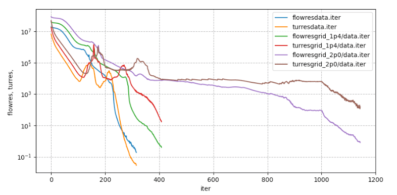
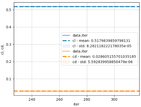
As shown below, all simulations' flow/turbulence residual converge 7+/5+ orders of magnitude, and their standard deviations of lift and drag coefficient over the last 100 iterations are well below a count. The three levels required ~77, ~294, ~3890 CPU-hrs of computational time, respectively. For a discussion on the RANS solution settings choices and analysis, see the RANS tutorial.
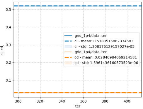
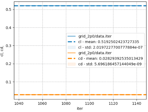
These plots were generated using LAVA's plotHist tool by running the
following commands in the run sub-directory:
plotHist.py -F                      data.iter iter cl cd -showStd -xRange  230  330
plotHist.py -F refinedGrid_1p414214/data.iter iter cl cd -showStd -xRange  300  400
plotHist.py -F      refinedGrid_2p0/data.iter iter cl cd -showStd -xRange 1040 1140
plotHist.py -F data.iter refinedGrid_1p414214/data.iter refinedGrid_2p0/data.iter iter flowres turres
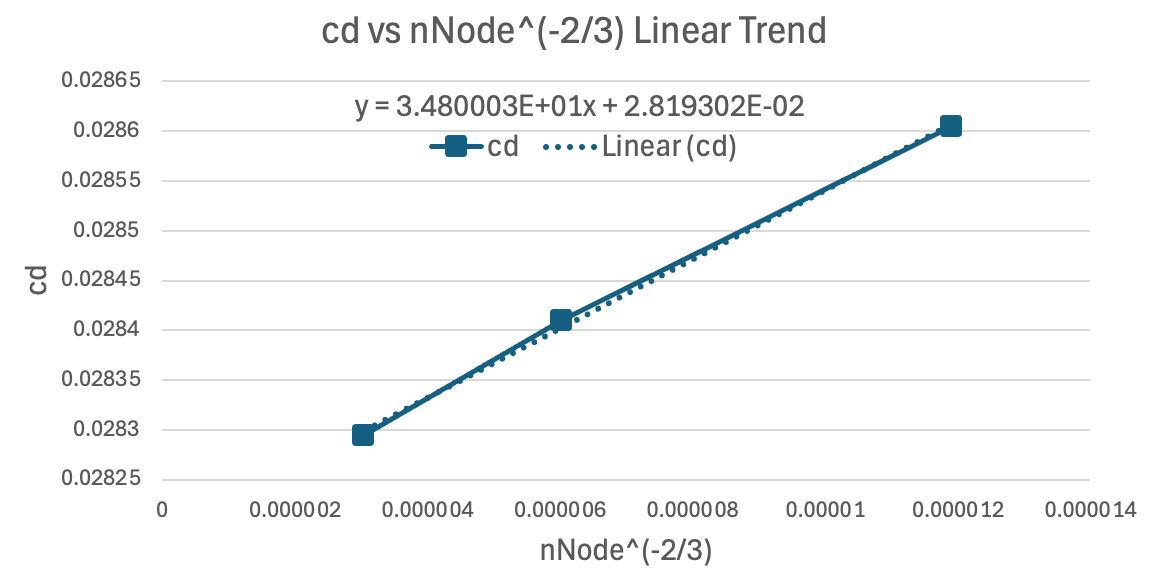
If we plot a trend of cd vs a linearized representation of 3D grid size
increase such that an infinitely fine grid is located on the x axis, we see a
very flat trend with an asymptotic cd estimate of 0.028193. Since all grids
are well within a defined linear trend and we can quantify the bounds of
integrated loads, it is safe to say that the initial grid is fine enough to
resolve the physics of the RANS case at AOA of 2.5 degrees.