Output and Probes
All the output settings are organized under output {} section.
Flow Stats
Controls interval of sampling flow statistics such as integrated kinetic energy, maximum Mach number and integrated domain volume (see Monitor section for descriptions).
Monitor
Monitor output tracks typically high frequency information such as time step, CFL, residuals, integrated aerodynamics loads and performance metrics among others.
If monitor section is not included in the input file, you will get a default set of variables output to screen every time steps (or every pseudo step for implicit runs). The variable list given here only affects the screen output while every other available variable is always output to the .iter file.
The .iter file can be plotted using the tool plotHist.py
output {
    monitor {
        # Output interval applies both to screen and file (.iter) file outputs.
        interval = 10
        # Variable list only affects the screen output
        variables = [nt,time,ctu,dt,maxcfl,maxmach,cl_airplane,wallt,mups,elapsed]
        # When restarting, the code looks for a copy of the .iter file in the restart directory
        # corresponding to the time step you are restarting from. If the .iter file is missing,
        # by default the code will quit with an error message. The flag below, if activated, will
        # instead start a new .iter file from scratch
        reset if missing = false # default
        # The monitor keeps track of some averaged performance metrics. This entry will set the interval
        # for averaging. By default, it is set to 10xinterval (specified above)
        avg interval = 100
    }
}
Each screen line ends with notes on what happened since the previous line, name^N for N times: the outputs
written (volume, iso, surf, point, line, restart), the buffered outputs flushed (write-surf-buff-N,
write-iso-buff-N, N files) and, on unst GPU runs, dtoh-q and dtoh-qave when all of the solution or of its
time averages was copied from the device to the host, which takes a noticeable share of a step on large grids.
List of available monitor variables:
| Variable | Description | Units |
|---|---|---|
| nt | Time step | |
| ns | Pseudo time step | |
| time | Physical simulation time | [s] |
| ctu | Convective time unit | [non-dimensional time] |
| dt | Time step size | [s] |
| nts | Completed sync steps (sync-clock runs only, see the time section) | |
| dtratio | dt / sync dt (sync-clock runs only) | |
| substeps | RK sub-steps in the last completed sync step (sync-clock runs only) | |
| maxcfl | Maximum CFL number in the domain | |
| maxmach | Maximum Mach number in the domain | |
| integratedmass | Integrated mass of fluid in the domain | [kg] |
| integratedvolume | Integrated volume of the domain | [m^3] |
| integratedke | Integrated kinetic energy in the domain | [J] |
| nondim_integratedke | Non-dimensional integrated kinetic energy | |
| integratedxmomentum | Integrated x-momentum | [kg*m/s] |
| integratedymomentum | Integrated y-momentum | [kg*m/s] |
| integratedzmomentum | Integrated z-momentum | [kg*m/s] |
| integratedetotal | Integrated total energy in the domain | [ (kg/m^3)(m^2/s^2) ] |
| nondim_integratedetotal | Non-dimensional integrated total energy | |
| minpressure | min pressure in the domain | [Pa] |
| maxpressure | max pressure in the domain | [Pa] |
| minuvelo | min u-velocity in the domain | [m/s] |
| maxuvelo | max u-velocity in the domain | [m/s] |
| minvvelo | min v-velocity in the domain | [m/s] |
| maxvvelo | max v-velocity in the domain | [m/s] |
| minwvelo | min w-velocity in the domain | [m/s] |
| maxwvelo | max w-velocity in the domain | [m/s] |
| mintemperature | min temperature in the domain | [K] |
| maxtemperature | max temperature in the domain | [K] |
| mups | Average MUPS, averaged through the log interval | |
| mups_min | Minimum MUPS through the monitor log interval | |
| mups_max | Maximum MUPS through the monitor log interval | |
| mups_long | Average MUPS, averaged through the avg interval | |
| mups_long_min | Minimum MUPS through the monitor avg interval | |
| mups_long_max | Maximum MUPS through the monitor avg interval | |
| wallt | Wall time per time step, averaged through the log interval | [s] |
| wallt_min | Minimum wall time through the monitor log interval | [s] |
| wallt_max | Maximum wall time through the monitor log interval | [s] |
| wallt_long | Wall time (s), averaged through the avg interval | [s] |
| wallt_long_min | Minimum wall time through the monitor avg interval | [s] |
| wallt_long_max | Maximum wall time through the monitor avg interval | [s] |
| elapsed | Total elapsed wall time from beginning, including the restart history | [hr] |
| memory | CPU host memory usage on root MPI rank | [GB] |
| memory_gpu | GPU device memory usage on root MPI rank | [GB] |
Note
MUPS: Millions of Updates per Second, i.e. millions of cells advanced through a full time step per second
Integratrated loads, as described in the Loads section, are also output via the monitor. Each loads integration group, corresponding to the its specied name will produce the following monitor output variables:
| Variable | Description |
|---|---|
| cx_name | Total x-force coefficient |
| cy_name | Total y-force coefficient |
| cz_name | Total z-force coefficient |
| cx_inv_name | Inviscid x-force coefficient |
| cy_inv_name | Inviscid y-force coefficient |
| cz_inv_name | Inviscid z-force coefficient |
| cx_visc_name | Viscous x-force coefficient |
| cy_visc_name | Viscous y-force coefficient |
| cz_visc_name | Viscous z-force coefficient |
| cmx_name | Total x-moment coefficient |
| cmy_name | Total y-moment coefficient |
| cmz_name | Total z-moment coefficient |
| cmx_inv_name | Inviscid x-moment coefficient |
| cmy_inv_name | Inviscid y-moment coefficient |
| cmz_inv_name | Inviscid z-moment coefficient |
| cmx_visc_name | Viscous x-moment coefficient |
| cmy_visc_name | Viscous y-moment coefficient |
| cmz_visc_name | Viscous z-moment coefficient |
| cl_name | Total lift coefficient |
| cd_name | Total drag coefficient |
| cs_name | Total side force coefficient |
| cl_inv_name | Inviscid lift coefficient |
| cd_inv_name | Inviscid drag coefficient |
| cs_inv_name | Inviscid side force coefficient |
| cl_visc_name | Viscous lift coefficient |
| cd_visc_name | Viscous drag coefficient |
| cs_visc_name | Viscous side force coefficient |
If running the implicit solver, there are a few additional monitor variables available:
Note
For residual norms ICOMP index below refers to the equation number:
0: Continuity, 1-2-3: Momentum, 4: Energy, >=5: Species mass fractions
For DQ norms, ICOMP index below refers to the primitive variables:
0: Pressure, 1-2-3: U-V-W velocity components, 4: Temperature, >=5: Species mass fractions
| Variable | Description |
|---|---|
| l0resICOMP | L0 Residual norm (absolute) |
| l2resICOMP | L2 Residual norm (absolute) |
| l0resrICOMP | L0 Residual norm (normalized by first step value) |
| l2resrICOMP | L2 Residual norm (normalized by first step value) |
| l0dqICOMP | L0 Primitive variable change norm (absolute) |
| l2dqICOMP | L2 Primitive variable change norm (absolute) |
| l0dqrICOMP | L0 Primitive variable change norm (normalized by first step value) |
| l2dqrICOMP | L2 Primitive variable change norm (normalized by first step value) |
| l0turbres | L0 Residual norm for turbulence equation (absolute) |
| l2turbres | L2 Residual norm for turbulence equation (absolute) |
| l0turbresr | L0 Residual norm for turbulence equation (normalized by first step value) |
| l2turbresr | L2 Residual norm for turbulence equation (normalized by first step value) |
| lambdap | Under-relaxation factor for Navier-Stokes equations |
| lambdatur | Under-relaxation factor for turbulence equation |
| lambdals | Under-relaxation factor for line search |
| linits | Number of linear solver (GMRES) iterations for Navier-Stokes equations |
| linres | Linear solver (GMRES) residual for Navier-Stokes equations |
| linitsturb | Number of linear solver (GMRES) iterations for turbulence equation |
| linresturb | Linear solver (GMRES) residual for turbulence equation |
Loads
In this section, you can define several loads integration groups which can integrate forces and moments over specified components of the geometry.
output {
    loads {
        # Interval at which the loads are computed, this is common for all integration groups
        interval      = 10
        # Following 3 inputs apply to all the groups by default
        # But you can optionally specify them different for any individual group
        # Center around which moments are computed
        moment center = [33.,0.0,4.5]
        # Provide non-dimensional force and moments
        normalize     = true
        # Use gauge pressure (p-p_ref) in pressure forces
        gauge         = true
        # If true, this flag will output each surface component integrations separately
        # (in addition to the groups listed below)
        do individual comps = true
        group_1 {
            # Group name
            name          = airplane
            # Which BC zones to include
            include       = [1-32]
        }
        group_2 {
            name = wing
            include = [7,8,10-13]
            normalize     = false
            # Use gauge pressure (p-p_ref) in pressure forces
            gauge         = false
        }
        group_3 {
            name = tail
            include = [14,16]
            moment center = [48.,0.0,4.5]
        }
        ...
    }
}
normalize = true is specified, the code will additionally output normalized force/moment coefficients. The values of the reference conditions section are used for normalization.
The result of the load integrations are output to screen (if requested) and to the monitor file (.iter). Detailed description of the monitor and the loads output variables are provided in the monitor section.
If you only have single loads integration group, you can skip the group_1 subsections:
output {
    loads {
        interval      = 10
        moment center = [33.,0.0,4.5]
        normalize     = true
        gauge         = true
        do individual comps = true
        name          = airplane
        include       = [1-32]
    }
}
Loads on moving bodies
In 3D, a loads group on a body moved by a rigid body motion block (rotation or translation, constant or sinusoidal) or lying in a non-inertial frame also reports its loads in the body's own axes and in its wind axes. The body of a group is the motion of the zones its walls belong to. A group holding walls of more than one body is reported with a warning; its body-axis loads stay in the reference frame and its wind axes come from the reference freestream. Groups on fixed walls keep the laboratory axes and write only the standard columns. In 2D the loads stay in laboratory axes.
- Body axes: the grid axes at the starting pose (x, y, z of the mesh as read), turned by the motion block's
initial attitudeif given, and then carried by the motion. In a non-inertial frame the grid axes are the body axes. - Moment centre: the group's
moment centeris a body-fixed point. The laboratory moments (Mx_<group>…) are taken about it as given, moved with a translation. The body-axis and wind-axis moments are taken about the point as the body has carried it. - Relative wind: the reference freestream (
alpha,betaand the reference velocity) minus the body's velocity at the moment centre (translation velocity plus Ω × r; in a non-inertial frame, the frame's Ω × r). - Wind axes: D along the relative wind, S the body y axis less its D part, L = D × S.
alpha_<group>andbeta_<group>are the angles of the relative wind in body axes, in degrees. With no relative wind, or the wind along the body y axis, the referencealphaandbetaare used.
| Monitor column | Meaning |
|---|---|
FL_<group>, FD_<group>, FS_<group> (and _inv_, _visc_) |
lift, drag and side force in the group's wind axes |
Fxb_<group>, Fyb_<group>, Fzb_<group> |
force in body axes |
Mxb_<group>, Myb_<group>, Mzb_<group> |
moment in body axes, about the carried moment centre |
Mroll_w_<group>, Mpitch_w_<group>, Myaw_w_<group> |
moment about D, S and L |
alpha_<group>, beta_<group> |
angles of the relative wind in body axes (degrees) |
C…b_<group>, CM…b_<group>, CMroll_w_<group> … |
the same, normalized, when normalize = true |
The body-axis and wind-axis moments are the same moment vector about the same point, split along different axes,
so their magnitudes agree. At beta_<group> = 0, S is the body y axis: Mpitch_w equals Myb, while roll and yaw
mix by the angle α (Mroll_w = Mxb cos α + Mzb sin α, Myaw_w = −Mxb sin α + Mzb cos α). The laboratory
moments Mx_<group> … are taken about the moment centre as given, so for a rotating body they also differ from the
body-axis moments by the shift of that point. D points downstream and L = D × S, so Mroll_w and Myaw_w have the
opposite sign to the flight-mechanics wind axes (x into the wind, z down); pitch has the same sign.
The columns below the standard ones are written only for groups on a moving body or in a non-inertial frame. A fixed
group's body axes are the laboratory axes, so its body-axis loads are Fx_<group> … Mz_<group>, and its wind axes come
from the reference free stream: the reference alpha and beta, or, when the reference conditions give phi or a
velocity vector, the angles of that velocity vector. Its FL, FD, FS follow that direction, and a wind-axis
moment is the laboratory moment projected on the axis, e.g. the roll moment about D = (cos α cos β, −sin β, sin α cos β):
Mroll_w = Mx cos α cos β − My sin β + Mz sin α cos β.
Two consequences, both checked to round-off: a model meshed turned in the grid and run with initial attitude set
to that turn reports the same loads as the unturned model at the matching alpha/beta; a body translating at a
constant velocity reports the same loads as the fixed body in the freestream of the matching relative wind. A
plunging aerofoil therefore reports the plunge-induced angle of attack in alpha_<group>.
Restart
Restart files, also referred to as checkpoint files, allow you to restart the simulation seamlessly from a given point. You can set the interval of restart file writes as:
output {
    restart {
        # Specify restart file output interval (time step for unsteady, pseudo-step for steady)
        interval = 1000
    }
}
Stopping a run early. Create a file named STOP in the run directory to end a run before its last step. The
solver looks for it every 40 steps and then ends the run after the step in progress (an implicit unsteady run
finishes its physical step, a subcycled Cart run its coarse step) as if it were the last one: it writes that step's
final outputs, every buffered output and a restart, and exits cleanly. A STOP file present when a run starts is
deleted.
When the scheduler ends a run. A batch scheduler ends a job past its wall time with SIGTERM, then SIGKILL after a
grace period. On SIGTERM to any rank, every rank writes its buffered outputs at the end of the step in progress and
the run exits with an error status, without a restart: a restart cut short by the SIGKILL could leave the latest
restart file unreadable. A second SIGTERM ends the run at once. To end with a restart, use a STOP file or set the
number of steps so the run ends before the job does.
Buffered surface outputs
Surface outputs (the BC surface output, the surface probes and the iso-surfaces) reach the disk in one of two ways:
- Gathered: the parts of an output on every rank are collected on one writer rank and written there as one file, in any format the output supports. Gathered outputs are buffered: an output is held in memory by a rotating storage rank and written at the next flush, so a flush writes many files from many ranks at once.
- Parallel: every rank writes its own part into one shared CGNS file, at every output, never buffered. A vertex that several ranks share is written once by each of them.
| Output | Unst | Cart |
|---|---|---|
| BC surface | gathered; doparallel = true in the surface section writes it in parallel |
gathered |
| Surface probe | gathered; doparallel = true writes it in parallel (format = cgns only) |
gathered |
| Iso-surface | gathered; doparallel = true writes it in parallel (format = cgns only) |
cgns and xdmf in parallel, vtk and vtp gathered; doparallel overrides |
On Unst, a gathered output whose single output, collected on its writer rank, would take more memory than the limit
below is written in parallel instead, as CGNS, for the rest of the run, so a large surface never has to fit on one
rank. The check is made once per output, at its first output with faces, and the log says which output it moved and
its size. A vtk or vtp output then writes .cgns files holding the same surface and values. Fwh and Plot3D
surface probes and Cart iso-surfaces have no parallel writer and stay gathered, with a warning.
Input (output section) |
Unit | Default | Effect |
|---|---|---|---|
output buffer interval surf |
steps | automatic | Flush the buffered BC surface and surface probe outputs every so many steps; 0 writes each output at once |
output buffer interval isos |
steps | automatic | The same for the gathered iso-surfaces |
output buffer snapshots |
outputs | 100 | The automatic intervals let each rank hold at most this many outputs |
output buffer flush period |
wall-clock seconds | 0 (off) | Also flush once the oldest buffered output has been held this long, which bounds what a killed job loses between restarts |
output buffer memory |
MB per rank, 1 MB = 2^20 bytes | automatic | Also flush at any output step that leaves a rank holding more than this; a single gathered output larger than this is written in parallel |
- The intervals count time steps; with a sync clock they count sync steps, and every output and flush happens on
the sync marks. The automatic interval is the number of steps over which all the buffered outputs, counted
together, fill
output buffer snapshotsoutputs per rank, and at least the number of ranks; it is shortened when the hosts are over half full at startup, and set to 1 over 80%. The log reports it. - Without
output buffer memory, the limit is a quarter of the memory available to each rank: the available memory of its node shared by the ranks on the node, the least over all ranks, measured when the check is made. The log reports it at the first surface output. - Every restart write, the end of the run, a
STOPfile and a SIGTERM flush every buffered output, so a restart never precedes outputs still in memory.
output {
    output buffer flush period = 1800 # flush at least every 30 minutes
    output buffer memory       = 2000 # flush once a rank holds more than 2000 MB
    surface {
        interval   = 100
        doparallel = true             # unst: every rank writes its part of each BC surface file
    }
}
Output file names
Snapshot files carry the output step in their name (the sync step when sync steps per ctu or sync dt is set),
and a link named after the same stem with Latest in place of the step points to the newest one. Probes are
numbered as their input sections are: surface probe_3 writes 003.*, line probe_12 writes 012.*, and the
lines of a multiline line probe file are numbered from 1 after the probe number.
| Output | Files | Latest link |
|---|---|---|
| Volume | volume/Unst.vol.<step>.cgns, subsets volume/sub<NN>.Unst.vol.<step>.cgns |
Unst.volLatest.cgns, sub<NN>.Unst.volLatest.cgns |
| BC surface | surface/Unst.surf.<step>.cgns |
surface/Unst.surfLatest.cgns |
| Iso-surfaces | isosurface/surf<NN>_<contour>[_isoVal<value>]_Color<fields>_<step>.<format> |
isosurface/surf<NN>_<contour>[_isoVal<value>]_Color<fields>Latest.<format> |
| Surface probes | surf_probe/<NNN>.Unst.<step>.<format> |
surf_probe/<NNN>.UnstLatest.<format> |
| Integrated quantities | surf_probe/<NNN>.mass_flux.dat, one history per probe |
|
| Line probes | line_probe/[<name>.]<NNN>[_<MMM>].Unst.<step>.line; binary: line_probe/[<name>.]<NNN>.Unst.line, one file per probe |
line_probe/[<name>.]<NNN>[_<MMM>].UnstLatest.line |
| Point probes | point_output/<NNN>.points.<variable>.dat, one history per variable |
|
| Restart | restart/Unst_restart.<step>.hdf5 |
restart/Unst_restartLatest.hdf5 |
The histories (point probe tables, integrated quantities) hold a row per output; a restarted run drops the rows from its first output step on before appending, so each output appears once.
Volume
Volume output writes the selected flow variables to a CGNS solution file at each output step, linked to a grid file that holds the grid.
The cells, faces and nodes of the volume and of its subsets (box and plane) are numbered in the order of the
grid's global ids, so the files hold the same grid and solution on any number of ranks. Each solution file
<prefix>.<step>.cgns (Unst.vol or sub<NN>.Unst.vol) links to a grid file <prefix>.meshLink.<step>.cgns, named
after the step of the first solution that uses it. A run links its solutions to the latest earlier grid file when
that file holds the same grid, recognized by a fingerprint of its contents stored in it, as on a restart on any number
of ranks; otherwise it writes the grid at its first output. A subset cutting moving zones writes a grid with every
output. The grid files hold the grid as the solver uses it, moved by the grid's transform inputs, and leave out
the nodes of the grid file that no face uses.
output {
    volume {
        # Whether to write out an volume file at the start of simulations (initial conditions)
        write initial = false
        # Currently only cgns format is supported
        format        = cgns # default
        # Interval of output (unsteady: time step, steady: pseudo-step)
        interval      = 10000
        # List of variables to output
        variables     = [q,qstats,density,mach,problem,sponge,upwind,cellmask,trip]
    }
}
In addition to the full volume output, you can also output a subset of the domain. Currently, two different types of subset are supported. They are described below along with the supporting options required:
box: Output all the cells inside a box defined by box vertices 'lo' and 'hi'. The 'lo' parameter defines the minimum x,y,z coordinates of the box, while 'hi' defines the maximum x,y,z coordinates.- On unstructured grids with zones that move with a rigid body motion, the box stays fixed in the lab: the cells are selected again at every output at their lab positions and written there, so every output of the subset writes its own grid file.
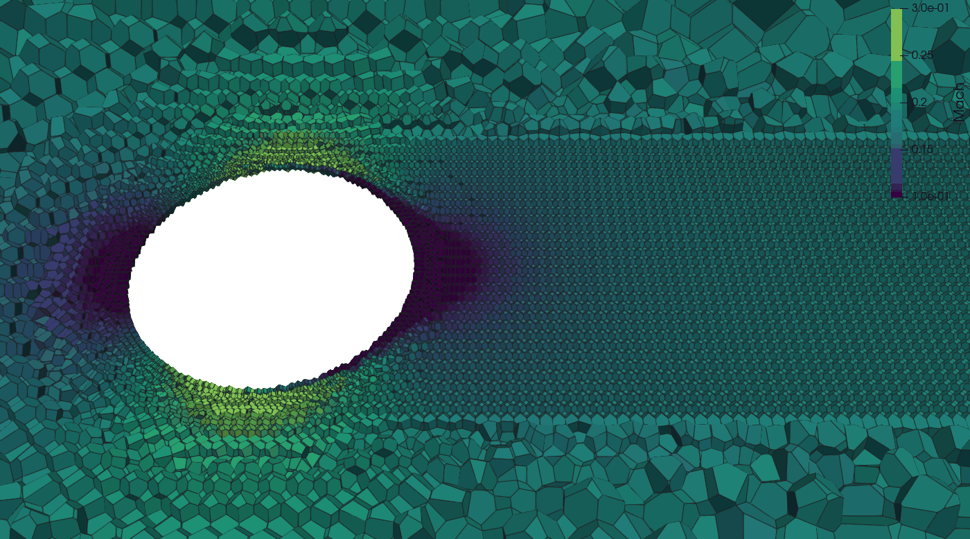
plane: Output the whole cells a plane passes through. The plane is defined bypoint, any point on the plane, andnormal, the direction perpendicular to the plane (it does not need to be normalized), as for surface probe and iso-surface cut planes.origin, the name of earlier releases forpoint, is still read with a deprecation warning. A cell is written when it has nodes on both sides of the plane, a node on the plane counting as the side opposite to the normal, so a plane lying on cell faces writes one layer of cells and a cell the plane only touches at a node or an edge is not written. A node counts as on the plane when it lies within the roundoff of its coordinates of it (2^16 units of roundoff, about 7e-12 of its coordinates' magnitude), as nodes a mesher meant to put on the plane do; the side of each node is decided exactly.cliploandcliphi(optional) keep only the cells whose centroid lies in that box.include zones(optional) restricts the cut to the listed grid zones, by CGNS zone name or 1-based index.- In a zone that moves with a rigid body motion, the plane stays fixed in the lab: the cells are selected again at every output and written at their lab positions, so every output of the subset writes its own grid file.
Where an iso-surface cutplane slices the cells into polygons and interpolates the solution onto them, a plane subset keeps the cells whole, with exactly the values the solver holds in each cell: use it to inspect mesh resolution, the tile and partition structure, or a stencil or a limiter cell by cell. ParaView calls this selection a crinkle slice and applies the same rule. To see the cells, open the file with the CGNS reader and show it as Surface With Edges.
  volume {
        # Whether to write out a volume file at the start of simulations (initial conditions)
        write initial = false
        # Currently only cgns format is supported
        format        = cgns # default
        # Interval of output (unsteady: time step or sync step, steady: pseudo-step)
        interval      = 10000
        # List of variables to output
        variables     = [q,qstats,density,mach,problem,sponge,upwind,cellmask,trip]

        subset_1 {
            type = box
            lo = [0.1, 0, 0.1]    # Minimum coordinates [x_min, y_min, z_min]
            hi = [1.0, 0.5, 1.0]  # Maximum coordinates [x_max, y_max, z_max]
            interval = 500        # Output interval specific to this subset
        }
        subset_2 {
            type = plane
            normal = [0, 0.5, 0.5]      # Direction vector perpendicular to the plane
            point  = [1.0, 0., 0.1]     # A point located on the plane
            cliplo = [-2.0, -0.5, -1.0] # (Optional) For clipping plane: Minimum coordinates [x_min, y_min, z_min]
            cliphi = [2.0, 0.5, 1.0]    # (Optional) For clipping plane: Maximum coordinates [x_max, y_max, z_max]
            interval = 100              # Output interval specific to this subset
        }
    }
The variables, write initial and format inputs are shared across all subsets. Each subset can have its own output interval that differs from the main volume interval. A subset's files are named after the volume's with sub<NN>. in front, NN the subset number: volume/sub01.Unst.vol.<step>.cgns on unstructured grids.
Tip
For large simulations, using subsets can significantly reduce storage requirements and post-processing time.
Full list of volume output variable options:
| Variable | Description |
|---|---|
| pressure | |
| velocity | All velocity components |
| temperature | |
| massfractions | Species mass fractions, only supported for multi-species |
| q | All of the above primitive flow variables |
| qstats | Time average and statistics of the flow field |
| density | |
| viscosity | laminar dynamic viscosity |
| nut | SA turbulence model working variable |
| eddyviscosity (or mut) | |
| mach | Mach number |
| umag | Velocity magnitude |
| vorticity | VorticityX, VorticityY, VorticityZ (or xvorticity, yvorticity, zvorticity for one) |
| vortmag | VortMag, the vorticity magnitude |
| qcriterion | QCriterion, 0.5 (|W|² - |S|²) of the velocity gradient |
| lambda2 | Lambda2, the middle eigenvalue of S² + W², negative in a vortex core |
| densitygradmag | DensityGradMag, the density gradient magnitude |
| distancefunction | Distance from walls |
| limiter | MUSCL slope limiter for each flow variable |
| upwind | Upwind/central blending sensor field, 0: central, 1: upwind |
| volume | Volume of each cell |
| dx | Cell size, the cube root of the cell volume |
| centroid | All 3 centroid coordinates for each cell |
| lsmooth | Smoothed length scale for each cell |
| residuals | All residuals (implicit only) |
| massresidual | Continuity equation residual implicit only |
| xmomresidual | X-momentum residual (implicit only) |
| ymomresidual | Y-momentum residual (implicit only) |
| zmomresidual | Z-momentum residual (implicit only) |
| energyresidual | Energy equation residual (implicit only) |
| nutresidual | SA turbulence model residual |
| dtau | Pseudo-time step size |
| sponge | Binary field indicating where sponging is active |
| trip | Binary field indicating where trips are active |
| thin | Binary field indicating whether a cell is marked as thin |
| problem | Binary field indicating whether a cell is marked as problem |
| problem_gg | Binary field indicating whether a cell failed Green-Gauss check |
| id | partition id for each cell |
| processor | rank owning each cell |
| tiles | tile id for each cell |
| domain | domain id for each cell |
| motion | motion id for each cell (-1: stationary) |
| cellmask | Cell bit mask |
Surface
Surface output writes one CGNS file per output, surface/Unst.surf.<step>.cgns, with a zone per boundary condition,
BC_<n>:<name>, holding its faces as polygons and the selected variables at the faces in solution solution;
include bcs limits the zones to the listed BCs (numbered from 1). A file holds the state of the step in its name,
and the faces of moving zones are where they are at that step. The files are gathered on rotating ranks and buffered
like the surface probes, written at the next flush, or with doparallel = true written in parallel by every rank (see
Buffered surface outputs); output buffer interval surf = 0 writes each gathered one at once.
With split grid and solution = true, the geometry goes in a grid file written at the first output of the run,
Unst.surf.meshLink.<step>.cgns after the step of that output, and each solution file links to the grid file of its
run. The linked geometry is that of the run's first output, also for
moving zones.
output {
    surface {
        # Whether to write out an initial file at the start of simulations (initial conditions)
        write initial = false
        # Interval of output (unsteady: time step, steady: pseudo-step)
        interval      = 10000
        # List of variables to output
        variables     = [q,qstats,density,mach,cf,yplus]
        # Link the solution files to a grid file written once per run instead of holding the geometry
        split grid and solution = false
        # The only format of the unstructured surface output
        format        = cgns
    }
}
BC Statistics Output
At every surface output step, area-averaged boundary condition statistics are appended to surface/bc_stats.iter, a continuous binary file in the same format as monitor/unst.data.iter. A human-readable mapping of BC indices to names is written once to surface/bc_name_map.txt.
The following quantities are recorded per boundary condition (prefixed BC1_, BC2_, etc.):
| Column | Description |
|---|---|
step, time |
Simulation step and time |
BCN_area |
Total boundary face area (m²) |
BCN_pressure |
Area-averaged pressure (Pa) |
BCN_u, BCN_v, BCN_w |
Area-averaged velocity components (m/s) |
BCN_temp |
Area-averaged temperature (K) |
BCN_y0, BCN_y1, ... |
Area-averaged species mass fractions (multi-species only) |
BCN_mach |
Area-averaged Mach number |
BCN_mdot |
Area-averaged mass flux (kg/(m²·s)) |
BCN_tauw_x/y/z |
Area-averaged wall shear stress components (Pa) |
BCN_heatflux |
Area-averaged heat flux (W/m²) |
BCN_hflux_min, BCN_hflux_max |
Min/max heat flux over the boundary (W/m²) |
When mach-driven pressure BCs are active, per-BC pressure history is written to surface/mach_driven_pressure_BCN.iter with columns step, mach_ave, pressure_ave.
Both bc_stats.iter and mach_driven_pressure_BCN.iter support restart continuation: history is automatically preserved across restart segments.
Full list of surface output variable options:
| Variable | Description |
|---|---|
| pressure | |
| velocity | All velocity components |
| temperature | |
| massfractions | Species mass fractions, only supported for multi-species |
| q | All of the above primitive flow variables |
| density | |
| mach | Mach number |
| viscosity | laminar dynamic viscosity |
| conductivity | thermal conductivity |
| specificheat | Cp |
| dtau | Pseudo-time step size |
| mdot | Mass flux (kg/(m^2.s), positive: inflow) |
| qdot | Heat flux (W/m^2, positive: inflow) |
| tauw | Wall shear stress (vector components) |
| cf | Surface skin friction coefficient (vector components) |
| pcoef | Surface pressure coefficient |
| yplus | Wall yplus value (zero on boundaries other than walls) |
| nut | SA turbulence model working variable |
| facemask | Face bit mask |
| cellmask | Cell bit mask |
| qavg | Time-averaged primitive flow variables |
| qstats | Time average and statistics of the flow field |
| tauwavg | Time average of wall shear stress (vector components) |
| yplusavg | Time average of wall yplus value (zero off walls) |
| turbulence | Turbulence sensor |
Iso-Surfaces
In-situ extraction of iso-surfaces for post-processing and visualization is supported. Iso-surfaces are defined by specifying a contour value for a chosen field, and the solver will output the corresponding isosurface as a triangulation at a user-defined interval.
isosurfaces_1 {
    isovalue     = 0.5
    contour      = vortmag
    colorfields  = [umag]
    interval     = 100
    format       = vtk
    clipbox_1 {
        lo     = [0.0, 0.0, 0.0]
        hi     = [1.0, 1.0, 1.0]
        invert = false
    }
}
isosurfaces_2 {
    contour      = cutplane
    normal       = [0, 1, 0]         # Normal vector of the plane (e.g., y-normal)
    point        = [0.0, 0.5, 0.0]   # A point on the plane
    colorfields  = [densitygradmag]
    interval     = 100
}
isosurfaces_3 {
    contour     = cutplane
    point       = [9.75, 0, 0]
    normal      = [1, 0, 0]
    format      = vtk
    interval    = 100
    colorfields = [q, mach, density]   # primary field first, then derived fields
}
isosurfaces_4 {
    isovalue        = 300
    contour         = q
    qcompcontouring = 4 # temperature component of the q vector for 3D simulations
    colorfields     = [q]
    qcompcoloring   = 0 # pressure component of the q vector
    interval        = 100
    format          = vtk
}
Parameters
- isovalue: The value of the chosen field at which to extract the iso-surface (e.g.,
isovalue = 0.5). - contour: The field to contour. Options include:
vortmag(vorticity magnitude, default)qcriterionlambda2machdensitygradmagq(a specific component of the q vector. The optionqcompcontouringis then required to specify the component index)cutplane(for planar cuts; requiresnormalandpoint, as surface probe cut planes and volume plane subsets do. On Unst, the whole cells a plane passes through are written by a volumesubsetoftype = plane)
-
colorfields: Array of fields to attach to the iso-surface, all written into the same output file. On Cart the first entry is the primary color field and any additional entries are derived variables (see the derived-variable list under colorfields (additional entries) below); on Unst the list is flat (see Unst color lists below). This replaces the need for several
isosurfaces_Nblocks that differ only in their color field, so one block produces one file per output interval instead of many (fewer inodes). The first entry may be:umag(velocity magnitude, default)vortmagqcriterionerrormetric(Cart only)densitygradmagmachdensitynut(Unst only; the turbulence model variable, needs a turbulence model)dx(cell size; on Unst the cube root of the cell volume)processor(the rank that extracted the vertex)inbody(Cart only; immersed-body indicator,1inside the geometry and0in fluid. On a cut plane the edge interpolation makes it a smooth0..1ramp across the body boundary, so you can threshold or mask on it. Most useful withdosolvecellsonly = false, the cut-plane default, so the plane fills through the body.)ducros(Cart only; Ducros shock/upwind sensordilatation²/(dilatation²+enstrophy)in[0,1], ~1 in compression/shocks, ~0 in smooth vortical flow — the sensor the CentralQ upwind blending uses)strain(Cart only; strain-based upwind sensor1 − enstrophy/(2·SᵢⱼSᵢⱼ+enstrophy)in[0,1], ~1 in strain/compression-dominated regions, ~0 in rotation-dominated flow)q(all components of the q vector; withqcompcoloring, only the component of that index.fullqis accepted as another name for all components)
On Cart, additional entries may be any of the same fields except
q, and require the first entry to beqwithoutqcompcoloring. Example:colorfields = [q, mach, inbody, ducros]. A single field with no extras is justcolorfields = [umag](or[mach],[inbody], etc.).Unst color lists. On Unst
colorfieldsis one flat list of up to 16 entries in any order:q,umag,vortmag,qcriterion,lambda2,densitygradmag,mach,density,nut,dx,processorandqstats. Each entry is written once, in the listed order, and the first entry names the file.qwrites all components of the q vector, or withqcompcoloringonly the component of that index; a list holding both the full vector (fullq) and aqcomponent drops the component with a warning. The written names are those of Cart (Umag,VortMag,QCriterion,Lambda2,DensityGradMag,Mach,Density,Nut,DX,Processor) and the volume output's state names forq. A vertex on a partition boundary is extracted by every rank holding its edge, soProcessordiffers between its copies. Example — one cut plane with the mean and instantaneous flow and the gradient fields:isosurfaces_1 { contour = cutplane point = [0, 0, 0] normal = [0, 1, 0] interval = 100 colorfields = [q, vortmag, qcriterion, mach, qstats] }Deprecated: the older
colorfield = <field>(single value) plusderivedvars = [...]syntax still works, but is deprecated and will be removed in a future release; usecolorfields = [<field>, ...]instead.colorfield = Xis equivalent tocolorfields = [X], andcolorfield = fullq; derivedvars = [a, b]is equivalent tocolorfields = [q, a, b]. A deck using either key warns at startup with the exactcolorfieldsline to replace it with. - interval: Output interval in time steps (e.g.,interval = 100). - format: Output file format. Withdoparallel = trueevery rank writes its piece of the surface into one shared file; withdoparallel = falsethe surface is gathered on one rank and written there, buffered overoutputbufferintervalisosoutputs (see Buffered surface outputs). A format its write path cannot produce stops at input. - Cart:vtk(default),vtpandcgnsgathered;cgnsandxdmfdefault to parallel output, andvtkwithdoparallel = truewrites one ASCII file per rank. - Unst:cgns(default),vtkandvtp, gathered and buffered unlessdoparallel = true, which writescgnsin parallel. A gathered iso-surface too large for one rank is written in parallel instead. -vtkandvtpfiles hold single precision values;vtpis VTK XML PolyData with raw binary appended data. -vtpwrites VTK XML PolyData (.vtp) files with raw binary appended data. - dosolvecellsonly: (Optional, Cart only) Restrict extraction to solved fluid cells, skipping immersed-body (INBODY) and GCM ghost cells (which carry non-physical reference/image states). Field contours (vortmag,qcriterion, etc.) default totrue. Cut planes default tofalse, so the plane fills through the body and you can see the section of the geometry — pair with theinbodycolorfield to visualize or mask the solid. Setdosolvecellsonly = trueon a cut plane to restore the old behavior (a clean hole at the body, no in-body data). - nearwallgradients: (Optional, Cart only, expert) Near-wall treatment of the gradient-based contour fields (vortmag,qcriterion,lambda2,densitygradmag) at immersed bodies, whendosolvecellsonlymasking is on. By default (ghost) gradient fields extend all the way to the wall using the immersed-boundary image states.nearwallgradients = excludeinstead stands them off about one cell from the wall, so the derivative stencils never touch the immersed-boundary band. - cliplo, cliphi: (Optional, deprecated) Lower and upper bounds for spatial clipping of the iso-surface, specified as coordinate arrays. Defaults to the full domain. Equivalent to a singleclipbox_1 { lo=...; hi=...; invert=false }; emits a deprecation warning at run time. Cannot be combined with indexedclipbox_Nsub-sections. Preferclipbox_1in new inputs. - clipbox_N: (Optional) Indexed axis-aligned box clip(s). Up to 4 boxes are supported per iso-surface (clipbox_1,clipbox_2, ...). Each box haslo,hi, and an optionalinvertflag (defaultfalse). Wheninvert=falsethe box keeps points inside it; wheninvert=trueit keeps points outside it. All configured boxes are AND'd together, and AND'd with allclipfrustum_Nregions. On Unst, boxes and frustums are in the coordinates ofpointandnormal(the laboratory frame, or the reference frame withframe = <zone>), and cells of moving zones are tested at their current position. Example — keep points inside a large box but excluded from a small interior box:- clipfrustum_N: (Optional) Indexed frustum (or hollow frustum) clip(s). Up to 4 frustums are supported per iso-surface (clipbox_1 { lo = [0.5, 0.0, 0.3]; hi = [1.0, 0.5, 0.7]; invert = false } clipbox_2 { lo = [0.7, 0.2, 0.45]; hi = [0.8, 0.3, 0.55]; invert = true }clipfrustum_1,clipfrustum_2, ...). The frustum axis runs fromlotohi;radiusis the cross-section radius atlo, and the optionalradiushiis the radius athi(defaults toradius, i.e., a cylinder). The optionalradiusinnerandradiushiinnercarve out a coaxial hollow region (defaults:0). An optionalinvertflag (defaultfalse) flips the keep/discard sense for that frustum: withinvert=truepoints inside the frustum are discarded. All frustums are AND'd together and AND'd with any box clips. Example — a hollow cylinder along the y-axis betweeny=0.1andy=0.4with outer radius0.18and inner radius0.08:- normal, point: (Optional) For planar cuts, specify the normal vector and a point on the plane.isosurfaces_4 { isovalue = 10 contour = vortmag colorfields = [umag] interval = 100 clipfrustum_1 { lo = [0.75, 0.10, 0.50] hi = [0.75, 0.40, 0.50] radius = 0.18 radiusinner = 0.08 # radiushi = 0.18 # optional, defaults to radius (cylinder) # radiushiinner = 0.08 # optional, defaults to radiusinner # invert = false # optional, default false } }
- include zones: (Optional, Unst only) Restrict extraction to the listed grid zones of a multi-domain grid, e.g.
include zones = [rotor1]. Entries are zone names as printed by the solver at grid read (1-based domain indices also work). Default: all zones. Tiles outside the listed zones are skipped entirely, so a tight filter also reduces extraction cost and file size. Applies to cut planes and field contours alike, and combines with box/frustum clips.
- frame: (Optional, Unst only,
cutplanecontour only, defaultlab) Reference frame the cut plane is fixed in. Withframe = <zone name>(a rotating zone, e.g.frame = rotor1;motion_Nalso works) the plane co-rotates with that zone's rigid body motion, so every output cuts the same material section of the blade.pointandnormalare interpreted in the chosen frame. With multiple rotors, each cut plane picks its own frame; zones with other motions appear at their instantaneous position relative to the reference frame. The defaultlabkeeps the plane fixed in the laboratory frame.
- frame coordinates: (Optional, Unst only, requires a rotating
frame, defaultlab) Coordinate system the extracted surface is written in.labdumps the vertices at their physical position, so the cut sweeps around with the blade and overlays volume, surface and iso-surface output directly — nothing to do in the viewer.frame = frameinstead writes them in the reference frame's coordinates: the blade and the cut then stand still across outputs while the far field counter-rotates (the blade-fixed animation), at the price of needing a viewer-side rotation to get back to lab coordinates. Either way the file records the frame state in aLAVA_FrameMotiondescriptor on the surface zone.
- relative velocity: (Optional, Unst only, default
false) With a rotatingframe, subtract the reference frame's rigid-body velocity from the velocity before computing the colors, so they show the flow as seen from the rotating frame. It applies to the velocity fields ofcolorfields(q, orqwith a velocity component,umagandmach), and the list must hold one of them; the gradient fields (vortmag,qcriterion,lambda2) use the velocity gradient in the laboratory frame. - writequads: (Optional, Cart only, default
true) For an axis-alignedcutplane(normal parallel to a coordinate axis), emit the surface as the connected quad mesh of the cut cells — one cell-footprint quad per sampled point, with the sampled values carried as cell-centered data — so the output visually matches the Cartesian grid and neighboring quads share corners (visualization tools can then compute gradients). Setwritequads = falseto keep the raw marching-cubes triangulation. Has no effect for non-axis-aligned planes or field contours, which are always written as triangles. - writeboxes: (Optional, Cart only, default
true) For an axis-alignedcutplane, write the outlines of the AMR boxes the plane passes through to a companionboxes_<filename>in the same directory — one quad per box, at the box's full extent, carryingProcessor,DXandLevelas cell data. Useful for seeing the domain decomposition and the AMR level structure behind a cut plane. The outlines come from intersecting the plane with the solver's real boxes, so this is independent ofwritequadsand needs no color fields. One is written alongside every cut-plane output, so each surface file has aboxes_file of the same timestep next to it — including when the plane produces no surface at all (e.g. one lying entirely inside a body), since the outlines come from the grid, not the surface. Has no effect on non-axis-aligned planes, field contours, or formats other thanvtk/vtp. Setwriteboxes = falseto suppress the companion file. - qcompcontouring: Required for
contour = q, selects the q component to contour. - qcompcoloring: Optional with a
qcolor field, selects the single q component to write; without itqwrites all components. -
colorfields (additional entries): The entries after the first in
colorfieldsare extra color fields written into the same file (except forqstats, the first entry must beqwithoutqcompcoloring). Available options are any combination of:qstats(Unst only; follows any first entry): the volume time average interpolated to the surface (pavg, uavg, vavg, wavg, tavg, TotalPressureAvg, pppp, upup, vpvp, wpwp, tptp, upvp, upwp, vpwp, as the volumeqstats), written after the other color fields. Requires atime averagingsection; listing it switches the volume average on likevariables = [qstats]in the volume block does. The fields hold zeros until the average starts. Typical use is a cut plane carrying the mean flow, e.g.colorfields = [q, qstats]. Averages added by a runtime input change need a restart.machdensityerrormetric(Cart only; contains zeros unless the solution-based AMR error-metric machinery is configured)densitygradmagumagvortmagqcriterionlambda2nut(Unst only)dx,processorinbody(Cart only; immersed-body indicator0..1, see the primary-field list above)ducros(Cart only; Ducros shock/upwind sensor[0,1])strain(Cart only; strain-based upwind sensor[0,1])
The output columns follow the order the fields are listed in
colorfields(on Cart the full q vector first when the primary isq, then each additional field in order, with theqstatsfields last; on Unst exactly the listed order). On GPUs, each additional field adds to the extraction kernel's shared-memory footprint; if the run aborts with a shared-memory error during isosurface setup, split the fields across two blocks. Cart example — one cut plane carrying the full state vector plus four extra fields in a single file (for Unst, droperrormetricand useformat = cgns):
Multiple Iso-Surfaces
You can define multiple iso-surfaces by incrementing the section name, e.g., isosurfaces_1, isosurfaces_2, etc.
Notes
- Cut planes need both
normalandpoint. - A cut plane that misses the grid or the domain is skipped with a warning at startup. On Unst this applies to cut planes in the laboratory frame on grids that do not move.
- On Unst the iso-surface is marched over a tetrahedralization of the cell centroids. A centroid whose value equals the iso value within roundoff, as on a cut plane through a layer of centroids of a lattice or mirrored grid, or a contour at the value a field holds over a uniform region, lies on the surface: the surface passes through it once, without zero-area triangles around it.
- On Cart,
cgnsandxdmfdefault to parallel output (doparallel = true), the others to a write from the gathered surface; on Unst every format defaults to the gathered write. - If the primary color field is
qandqcompcoloringis not specified, the full Q vector is used for coloring. - Buffered output for isosurfaces is controlled by the
outputbufferintervalisosvariable in the output section, which defaults to an interval the code determines (see Buffered surface outputs). Buffering applies to gathered output; on Cart an iso-surface written in parallel turns it off for all of them (with a warning whenoutputbufferintervalisoswas set), on Unst it leaves the others buffered. - For
qcompcontouringandqcompcoloring, the component of the state vector follows this 0-index order: [p u v (w) T (Y1 Y2 Y3 ...)]. Here, note that the fieldwonly exists when running the 3D executable.
Note
LAVA unstructured writes iso-surfaces as cgns (the default), vtk or vtp, gathered on one rank and buffered; doparallel = true writes a cgns iso-surface in parallel by every rank (see Buffered surface outputs). The errormetric contour and color field are not supported.
Note
An iso-surface file holds the solution of the step in its name: _000000000 is the initial condition.
Note
Iso-surfaces and cut planes are extracted on CPU runs as well as on GPU runs. On CPU runs the tiles are tetrahedralized once at startup and the surfaces are extracted with marching tetrahedra.
Surface Probe
Surface probes sample the flow on a cut plane or on a triangulated surface read from a file. Each probe is
written to its own file in the surf_probe directory at its interval, named as in
Output file names. Every file holds its grid and its solution.
By default, surface probes sample the primitive flow variables (p, u, v, w, T, Y) and, in a turbulent run, the
turbulence variable; variables selects others (see Probe variables). Every probe writes an InOut variable: 1 where the value was found
inside the mesh, 0 for a point outside it, which takes the value at its nearest boundary point. On grids with moving zones, see
Probes and moving zones. The volume time averages of the run are added with
output qstats = true.
Cut planes
A cut plane is given by a point on it, point, and its normal, normal, in any direction and of any
length; numplanes evenly spaced parallel planes run from point to pointhi. Iso-surface cut planes and
volume plane subsets take the same point and normal. The names of earlier releases, cutpoint,
cutpointhi and cutdirection = x, y or z, are still read, with a deprecation warning that gives the
replacement line.
output {
    surface probe_1 {
        point    = [0, 0.1, 0]  # a point on the plane
        normal   = [0, 1, 0]    # the plane normal
        interval = 10
    }
    surface probe_2 {
        point    = [0.5, 0.5, 0.5]
        normal   = [1, 1, 1]       # any direction, of any length
        interval = 10
    }
    surface probe_3 {
        point        = [0, 0, 0.1]
        pointhi      = [0, 0, 0.9]
        numplanes    = 3           # planes evenly spaced from point to pointhi
        normal       = [0, 0, 1]
        interval     = 10
    }
    surface probe_4 {
        point        = [0, 0.1, 0]
        normal       = [0, 1, 0]
        crinkle      = true        # the mesh faces separating the two sides
        interval     = 10
    }
}
The plane cuts every cell it passes through into a polygon, so the polygons tile the plane's section of
the mesh with no gaps, across cells and ranks. A node on the plane counts as below it: a plane
lying on cell faces gives one polygon per face, from the cells above, and cells the plane only touches
at a node or an edge give none. A node within the roundoff of its coordinates of the plane (about 7e-12 of
their magnitude) counts as on it, so a plane through a layer of faces whose nodes the mesher stored up to
roundoff off the plane, such as a symmetry plane of a Voronoi lattice, still gives one polygon per face. A
plane through a moving zone is cut again at every output, at the zone's position at that time. The polygons of a probe with several planes are tagged by plane index in
the plane field.
With crinkle = true, the probe writes mesh faces in place of the polygons: the faces between a cut cell
and a cell entirely below the plane (every node below or on it), oriented toward the positive side. They
form a staircase within one cell below the plane, reaching the domain boundary, with no new geometry; a
plane on cell faces gives those faces.
The values are interpolated from the cell the plane cuts and its neighbours, by a least-squares fit that
is exact for a linear field: with the default data location = face at each polygon's centroid, and
with data location = node at the vertices. Crinkle faces are interpolated at their centroids from
their cut cell.
Note
Each cut cell gives one polygon per closed loop of its section. Faces whose edges do not match (a hanging node listed by one face but not by its neighbour) leave loose ends, which are joined; the run reports how many cells needed it. A cell whose section has a hole is written as the outer polygon and the hole as separate polygons, the hole oriented against the plane normal, so the hole's area is subtracted in the integrated quantities but shows filled in a viewer.
Surfaces read from a file
output {
    surface probe_5 {
        # Specify file, the format is determined by extension
        # Supported formats: tri, fro, cgns, vtk, p3d
        file = probe_triangulation.cgns
        interval = 100 # Interval of output
        # Where to sample data, either face center or nodes (vertices)
        data location = face # default, options: face, node
        # Optionally transform the probe triangulation. The operations are applied in the order: 1. rotation, 2. scale, 3. translate
        rotate = [90.,0.,0.]
        scale = [2.,1.,1.]
        translate = [1., 1. ,1.]
        format = cgns
        variables = [q, problem, sponge, upwind, limiter] # the flow and the cell status
        output integrated  = true # Output integrated quantities like fluxes through the surface probe
    }
}
The values are interpolated at the face centers or at the nodes. The component number of each triangle
is written in the component field.
Formats
The format option selects cgns or vtk for any probe; doparallel = true writes a cgns probe in parallel by
every rank instead of gathered (see Buffered surface outputs). Surfaces read from a file can also be written
as fwh, a specialized format for high frequency sampling of acoustic surfaces that holds only the face
values of p, u, v, w and T without the grid (it needs data location = face), or as p3d, a Plot3D
function file of the node values of p, u, v, w and T on the zones of a p3d input (it needs
data location = node).
Integrated quantities
Integrated quantities are requested by setting output integrated = true. Each probe keeps one history,
surf_probe/<probe index>.mass_flux.dat, with a row per output for every component of a surface read from a
file, or every plane of a cut plane probe. Its first line, starting with #, names the columns:
| Column | Quantity |
|---|---|
| 1 | Output step (the sync step when sync steps per ctu or sync dt is set) |
| 2 | Time |
| 3 | Component number, or plane index |
| 4 | Area |
| 5 | Mass flux |
| 6, 7 | Mass flux weighted total pressure and total temperature |
| 8 | Gross mass flux, the sum of the absolute mass flux of every face |
| 9, 10 | Mass flux weighted and area weighted Mach number |
| 11 | Area weighted pressure |
| 12-14 | Mass flux weighted velocity components |
| 15-17 | Area weighted velocity components |
A restarted run drops the rows from its first output step on and appends, so the history holds each output once.
The gross mass flux and the area weighted averages stay meaningful when the net mass flux is near zero. They are summed over the faces from the values
interpolated at the face centers, so they need data location = face, the default. The area of a cut
plane is its section's area along the plane normal (for crinkle faces, their area projected on it), and
the mass flux is positive along the normal.
Moving surfaces and rotating frames
The mass flux is the flux through the surface as it moves: at each face, the density times the velocity relative to the face, ρ (u − w) · A, where w is the velocity of the face at its center.
- A surface at rest in the lab has w = 0, and the mass flux is ρ u · A.
- A surface fixed in a moving frame (
frame = motion_Non a moving mesh, see Probes and moving zones) moves with that frame: w is the frame's velocity, Ω × r for a rotation and the translation velocity for a translation. - A face in the zones of a rotating non-inertial frame (
noninertial = true) turns with that frame, w = Ω × r, whatever frame the surface was given in. The mesh of such a frame does not move: its coordinates turn with the frame, so a surface placed in them turns too. A face in a stationary zone next to it, as on a plane crossing both, stays at rest.
This is the mass flux the solver conserves: its convective flux through every mesh face uses the same relative velocity, so the mass flux through a closed surface balances in a flow that is steady in the frame. Taken with the absolute velocity instead, the flux through a closed surface would not balance wherever the density varies, since ∮ ρ (Ω × r) · dA = ∫ (Ω × r) · ∇ρ dV. It also makes the result independent of how the rotation is modelled: a rotor run as a non-inertial frame, and the same rotor run on a rotating mesh with the surface in its frame, give the same mass flux.
The weighted averages take this mass flux as their weight and average the absolute flow quantities: the total pressure, total temperature, Mach number and velocity are those of the flow in the lab, not relative to the surface. In the zones of a non-inertial frame, the velocity components are along the frame's axes, which turn with it.
Line Probe
lineprobe_1 {
    start = [-1.000, 0.0,0];
    end = [1.000,0.0,0];
    number of points = 512;
    interval = 20;
    # Optional: also write time-averaged statistics (means, RMS, Reynolds stresses)
    # alongside the instantaneous state. See the Time Averaging section for the schedule.
    variables = [q, qstats];
    }
Warning
By default, each line probe output is written to an ASCII formatted file with one file per time step. This can quickly generate numerous files, potentially causing file system issues.
To mitigate this, a binary file format can be used by setting write binary to true. This creates a single binary file per line probe that contains data for all timesteps, significantly reducing the number of files created during your simulation.
For visualization and analysis, you can use the plotLineProbe.py tool, which is specifically designed to read and process these binary files.
When restarting simulations, the code handles existing binary line probe files:
- It checks if the current line probe definition matches the existing file
- If definitions match and restart time step is consistent, it simply appends new data
- If definitions match but restart time step differs, it creates a backup of the original file and prepends existing data up to the restart point in a new file
- If definitions don't match, it creates a copy of the existing file and starts a new file with the current definition
This robust handling ensures data integrity across simulation restarts while preserving your previous results.
Averaged quantities can be requested by setting the option output qstats to true.
output {
    line probe_1 {
        ...
        output qstats = true # Output averaged quantities sampled on to the probe
    }
}
Wall-Normal BL Probe
Line probes support a wall normal mode for boundary layer profiling. Instead of specifying a start/end pair, you supply one or more seed coordinates; the solver projects each seed onto the nearest no-slip or wall-function boundary face and grows a wall-normal ray of sample points outward to a specified height.
Seed specification — a single seed can be given inline with start; multiple seeds are read from a plain ASCII file (one x y z per line):
output {
    line probe_2 {
        wall normal = true
        file        = seeds.dat   # one "x y z" per line; omit to use start = [x,y,z]
        height      = 0.1         # outer extent of each ray in solver length units
        interval    = 500
        output qstats = true
        name          = bl_probe
    }
}
Ray discretization — choose one of two modes:
Uniform — evenly spaced points including the foot at h = 0:
Geometric — first cell height ds0, each subsequent step multiplied by growth rate (default 1.2) until height is reached; the final point is snapped to height. The actual number of points is determined automatically.
Optional keys:
| Key | Type | Default | Description |
|---|---|---|---|
wall bc names |
string list | all wall BCs | Restrict BVH projection to BCs matching these names |
flip normal |
bool | false | Flip the wall-outward normal direction |
output qstats |
bool | false | Include time-averaged quantities (requires volume time averaging) |
name |
string | line_probeN |
Base name for the output file |
Output file format:
BL probe files are written in Tecplot ASCII multi-zone format. One zone is created per seed; the zone title carries the 0-based seed index (T="seed_0", T="seed_1", …). Each zone header stores the projected foot coordinates as AUXDATA:
| AUXDATA key | Description |
|---|---|
x_foot, y_foot, z_foot |
Projected wall face centroid coordinates |
Data columns (one row per sample point):
nt time x y z [variables] InOut height tau_w_inst rho_w_inst mu_w_inst [tau_w_avg rho_w_avg mu_w_avg]
height— wall-normal distance from the foot (0 at the projected wall face centroid)tau_w_inst/tau_w_avg— instantaneous and time-averaged wall shear stress magnitude at the foot (constant within a zone)rho_w_inst/rho_w_avg— density at the foot, instantaneous and time-averagedmu_w_inst/mu_w_avg— dynamic viscosity at the foot, instantaneous and time-averaged- Avg columns (
tau_w_avg,rho_w_avg,mu_w_avg) are present only whenoutput qstats = true
On the first output step, two Tecplot equation files are written to the line_probe/ directory:
bl_inner_scale_inst.eqn— computesu_tau,nu_w,y+,u+,v+,w+from the instantaneous foot columnsbl_inner_scale_avg.eqn— same using_avgcolumns; also adds<uu>+through<vw>+from qstats
Load via Data → Alter → Specify Equations → Load in Tecplot.
Point Probe
Point probes will sample the flow state at a number of given points.
A group of points can be specified at once using an ascii file that lists the x y z coordinates of each point in order (space delimited):
output {
    point probe_1 {
        file = ascii_file_with_xyz_coords.dat
        interval = 1 # Interval of sampling
        scale = 1 # Option to scale the coordinates
        # Optional: also write time-averaged statistics (means, RMS, Reynolds stresses).
        # See the Time Averaging section for the schedule.
        variables = [q, qstats]
    }
}
Results will be written to an ascii file in the point_output directory, where each probe section and each variable will get its own file.
Alternatively, points can be output to the iter file and be plotted using plotHist.py tool by:
By default, point probes sample the primitive flow variables(p,u,v,w,T,Y_i), and variables selects others
(see Probe variables), along with an InOut variable indicating whether the query point was detected inside the fluid domain or out. A point outside the domain takes the value interpolated at its nearest boundary point, from the boundary cell and its BC ghost; line probes do the same. Optionally, you can output the Mach number as:
Averaged quantities can be requested by setting the option output qstats to true.
output {
    point probe_1 {
        ...
        output qstats = true # Output averaged quantities sampled on to the probe
    }
}
Probe variables
Point, line and surface probes write the variables their variables list names, in its order, followed by
InOut unless the list places inout elsewhere:
| Entry | Written as | Source |
|---|---|---|
q (default) |
Pressure, UVel, VVel, WVel, Temperature, MassFraction_\<species> | interpolated |
pressure, velocity, uvelocity, vvelocity, wvelocity, temperature, massfractions |
the corresponding part of q |
interpolated |
nut |
Nut (Spalart-Allmaras) | interpolated |
qstats, qavg, pavg, ..., reynoldsstress, tke, totalpressureavg |
the volume time averages: pavg, uavg, ... | interpolated |
density, rho |
Density | from the interpolated state |
mach, machnumber |
Mach | from the interpolated state |
umag |
Umag | from the interpolated state |
viscosity, mu |
Viscosity | from the interpolated state |
conductivity, lambda |
Conductivity | from the interpolated state |
specificheat |
SpecificHeat (at constant pressure) | from the interpolated state |
soundspeed, sound |
SoundSpeed | from the interpolated state |
totalpressure, ptot |
TotalPressure (isentropic) | from the interpolated state |
problem, sponge |
problem, sponge: 1 in a problem cell or a sponge zone, 0 elsewhere | interpolated |
upwind |
upwind: the upwind blend weight, averaged over the cell's faces | interpolated |
limiter |
limiter_0, ..., limiter_\<NUMQ-1>: the limiter of each primitive variable, averaged over the cell's faces | interpolated |
vorticity, xvorticity, yvorticity, zvorticity |
VorticityX, VorticityY, VorticityZ | interpolated gradient field |
vortmag |
VortMag | interpolated gradient field |
qcriterion |
QCriterion | interpolated gradient field |
lambda2 |
Lambda2 | interpolated gradient field |
densitygradmag |
DensityGradMag | interpolated gradient field |
volume |
volume: the volume of the cell holding the point | the cell's |
dx |
DX: the size of the cell holding the point, the cube root of its volume | the cell's |
inout |
InOut | 1 inside the mesh, 0 outside |
output {
    point probe_1 {
        file      = points.dat
        variables = [pressure, density, mach] # writes Pressure, Density, Mach and InOut
    }
}
The derived variables are evaluated from the interpolated pressure, velocity, temperature and mass fractions,
which are first kept within their bounds; for a field that varies linearly, the interpolated state is exact.
The time averages are those of the volume averaging, so they need a time averaging block; they are zero
until the averaging starts. Any other entry stops the run. The file and column names are the volume output's
(Mach, InOut, Nut, MassFraction_<species>). Binary point probe files (.q) hold the primitive
variables, and their .qstats companions the time averages, whatever the list.
A surface probe whose files feed a distributed boundary condition must hold the primitive variables and then the
turbulence variable, in that order, which its default list does; an explicit list has to start with q, nut.
The gradient fields (vorticity, vortmag, qcriterion, lambda2, densitygradmag) are evaluated in each cell
from its gradient stencil, the one the solver reconstructs with, in the laboratory frame: the vorticity components
are those of the lab axes in moving zones too. They are computed only at the steps an output lists them, and only
the fields listed; probes interpolate the cell values. S and W are the symmetric and antisymmetric parts of the
velocity gradient. In a cell beside a wall the gradient includes the BC ghost state.
The cell status (problem, sponge, upwind, limiter) comes from the residual of the step the probe samples
in, at the state the probe samples. output cell status = true on a surface probe is deprecated: it adds the four
entries the list lacks, with a warning. The interpolated cell status is kept between 0 and 1, the range of every
cell's flags and blend weights, where the fit overshoots between cells.
volume and dx are those of the cell holding the point, as the volume output writes them, not interpolated; a point
outside the mesh takes the boundary cell its values come from, and a point on a face between two cells takes one
of them.
Probes and moving zones
On a grid with zones moved by a rigid body motion, every point, line and surface probe is fixed in a frame,
set with frame:
lab(the default): the probe stays where it is in the lab. A point inside a moving zone samples whichever cell of that zone passes over it at the output time.motion_N, or the name of a moving zone: the probe moves with that motion. Its coordinates are given in the zone's own (stored) coordinates, those of the grid file, and it samples the same place of the zone at every output. Points in other zones, which move relative to it, are located again at every output.
output {
    point probe_1 {
        file  = rotor_points.dat
        frame = motion_1 # the points turn with motion_1
    }
    line probe_1 {
        start = [0.2, 0, 0]
        end   = [0.8, 0, 0]
        number of points = 31   # frame = lab by default: the line stays in the lab
    }
}
In the zones of a rotating non-inertial frame (noninertial = true), the mesh does not move and its coordinates
are those of the frame, which turn with it. A probe point there therefore stays at rest in that frame, whatever
frame it is given: a point cannot be held still in the lab in coordinates that turn. The run warns when a probe
given in another frame has points or faces in such zones; frame = motion_N, naming the non-inertial frame's
motion, states it and silences the warning. For the mass flux of surfaces in those zones, see
Moving surfaces and rotating frames.
Cost
A point is found once, at setup, in the zones at rest in its frame. A point covered by a zone that moves
relative to its frame is located again at every output: a search over that zone's cells, a new
interpolation stencil and a reduction over the ranks. The cost grows with the number of such points, not
with the grid, but a probe in the lab frame with many points inside moving zones costs more per output than
the same probe in the zones' own frame (motion_N), whose points are found once.
- Written coordinates: ASCII line probe files and surface probe files give each point at its lab position at the output time. Binary line probe files keep the coordinates given, in the probe's frame, in their header.
- Cut planes (
surface probewithpoint): a plane in a moving frame turns with it and is sliced again at every output. - Wall-normal line probes follow the zone of their wall, whatever its motion;
framedoes not apply to them. - Integrated quantities of a surface probe need a surface at rest in the lab.
relative velocity, which Cartesian probes accept, is not available for unstructured probes.
Time Averaging
Time averaging accumulates running statistics of the flow (means, RMS of the fluctuations, Reynolds shear stresses, mean total pressure, ...) as the simulation advances. Two things are configured independently:
1. Which averaged quantities are written. Add the averaging tokens to the variables list of
the output you care about (volume, surface, or a line/point probe). Each token expands to its
averaged columns:
| token | averaged columns |
|---|---|
qavg |
means of pressure, velocity, temperature (and species) |
qstats |
the full statistics set: the qavg means, mean total pressure, RMS of each fluctuation, and the Reynolds shear stresses |
yplusavg (unstructured surface) |
mean y+ |
tauwavg (unstructured surface) |
mean wall-shear-stress components |
Volume (and unstructured surface) second moments are central moments, the averages of the
fluctuations: pppp, upup, vpvp, wpwp, tptp and upvp, upwp, vpwp hold p'p', u'u', ...
and u'v', ...; do not subtract the squared mean. A moment is always written with its mean.
Cartesian surfaces and probes take qstats only (a partial token is an input error). Line
probes, point probes, the body surface and each surface probe accumulate the statistics on their
own sample points and write them as extra columns of their ordinary output files:
pavg uavg vavg wavg tavg TotalPressureAvg prms urms vrms wrms trms uvavg uwavg vwavg. A surface
also gets the running mean of every other column it writes, named <column>avg (Machavg,
Densityavg, yplusavg, qdotavg, tauwXavg, MassFraction_<species>avg, ...; not turbulence
or ReactionStepCount), and the rms of the wall shear (tauwXrms, tauwYrms, tauwZrms). The statistics survive regrids, moving-body re-clips and
restarts at any rank count; every vertex shares its surface's averaging window, newly exposed
surface takes the history of the nearest carried surface, and probe vertices inside a body hold no
statistics. output qstats = true in a surface or surface probe block is the same as listing
qstats.
2. When and how often to accumulate. The optional time averaging { } block sets the
schedule. A global schedule applies to every target; per-target sub-blocks override it. If the
block is omitted entirely, averaging begins at the first step and samples every step.
output {
    time averaging {
        # ---- global schedule (inherited by every target) ----
        # Start averaging at a step, physical time, or CTU (specify only one).
        # If none is given, averaging starts at the first step.
        start ctu = 50
        # Fold a sample into the running average every N steps. Default: the loads interval, or 100
        # without loads output.
        sampling interval = 1
        # cumulative (default) | exponential   (see "Exponential Moving Average" below)
        method = cumulative

        # ---- optional per-target overrides ----
        volume      { sampling interval = 10 }  # average the volume less frequently
        surface     { start ctu = 60 }          # start the surface average later
        lineprobes  { sampling interval = 1 }   # (Cartesian) probe-statistics schedule
        pointprobes { sampling interval = 1 }
    }

    volume  { interval = 1000; variables = [q, qstats] }               # write cadence + averaged columns
    surface { interval = 1000; variables = [q, wallmodel, qstats] }    # Cartesian: qstats columns
}
Key points:
- The start is inclusive. The first sample is the solution at the start step, or at the first step at or after the start time or CTU, and every output holds the samples up to and including its own step.
- The sampling interval is independent of the output
interval.sampling intervalcontrols how often a sample is folded into the running average; the outputintervalcontrols how often the current average is written to disk. Averaging accumulates continuously at the sampling cadence regardless of when files are written. - When no
sampling intervalis set, globally or in the target's own block, every target (volume,surface,lineprobes,pointprobes) samples on the loadsinterval, or every 100 steps when there is no loads output. Setsampling interval = 1to sample every step. - Listing an averaging token in a target's
variableslist is what enables averaging for that target; thetime averaging { }block only shapes the schedule. - Targets are
volume,surface,lineprobes, andpointprobes. Each inherits the global schedule and overrides only the keys it sets.
Exponential Moving Average
By default, LAVA uses a cumulative average (equal weight to all past samples). For long unsteady
runs it can be useful to instead use an exponential moving average (EMA), which gives a decaying
weight to older data so that the average tracks the recent flow statistics. Select it with
method = exponential and set a window:
time averaging {
    start ctu = 50
    method    = exponential

    # Window size W in CTU. Data older than W has approximately 3% residual weight.
    window ctu = 10
    # Alternatively, specify the window directly in physical time units (seconds):
    # window = 0.05
}
The EMA blending weight at each sample step is:
where \(W\) is the window size in physical time and \(\Delta t_\text{elapsed}\) is the elapsed physical time since the last averaging sample. At each step the average is updated as:
In the continuous limit, data from time \(\tau\) ago carries weight \(\propto e^{-c\,\tau/W}\). At exactly
one window back (\(\tau = W\)) the residual weight is \(e^{-3.5} \approx 3\%\). method and window may
be set globally or inside any per-target sub-block.
Legacy keys
Older input spellings are still accepted for backward compatibility:
do volume/do surface— deprecated and no longer needed. Volume and surface averaging are now controlled solely by whether averaging tokens appear in the target'svariableslist. For Cartesian surfaces,do surface = falsestill turns the surface statistics off.do exponential moving average = truewithexponential moving average window ctu(orexponential moving average window) — the pre-methodEMA spelling.frequency— deprecated alias forsampling interval.
Note
For unstructured line and point probes, time-averaged statistics are interpolated from the
volume average, so qstats on a probe requires volume time averaging to be active.