Overview
This material reflects the content presented by the LAVA team's tutorial during the 2026 Overset Grid Symposium. While intended as a follow-along for the in-person tutorial, this material is of value to new LAVA Curvilinear users as it showcases best-practices in how to think about gridding, scripting, solving on, and setting up optimization/design problems for an overset grid system.
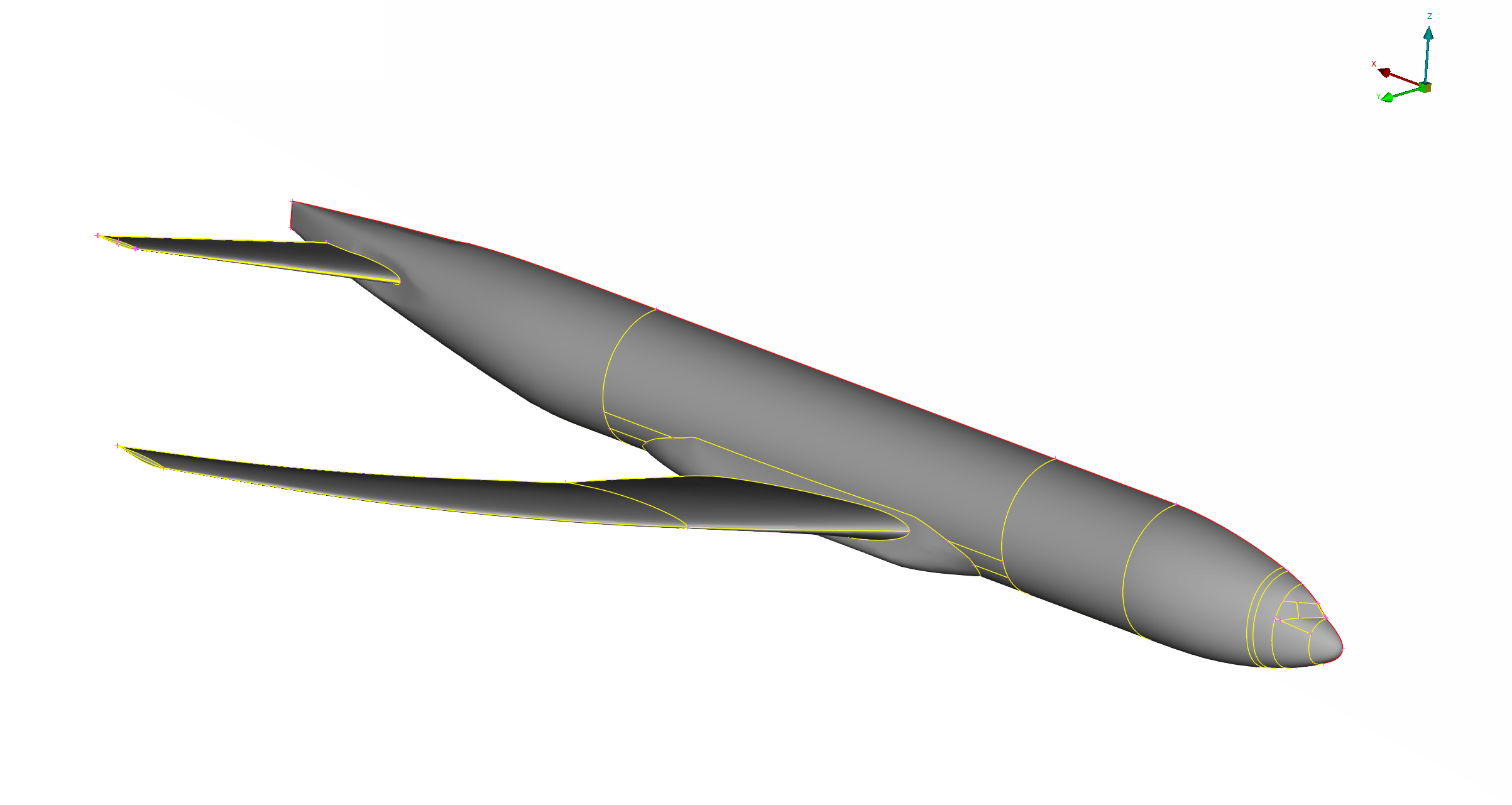
The baseline geometry considered is the Common Research Model (CRM) used in Drag Prediction Workshop 6. The initial wing and horizontal tail are added to in later tutorials to exemplify available design/optimization techniques.
Tutorial Set
The larger OGS tutorial has been broken into piecemeal tutorials which are intended to be completed sequentially, taking outputted files from previous tutorials as a starting point. However, 'checkpoint' files are provided within each tutorial to allow the user to start from any point.
The tutorials, along with what the user should expect to take away from them, are as follows:
- Project Grid Scripting
- How to setup component-based scripted grid generation for a LAVA Curvilinear project.
- What to consider when preparing CAD geometry for gridding.
- Rules of thumb for surface grid generation with forethought towards LAVA gridding utilities.
- How to use the octFarfield executable to create a farField which can then be connected to script-generated nearBody grids.
- Connecting a Grid
- How to connect a built curvilinear overset grid.
- Strategies for removing orphans.
- Generating a Grid using EPOGS
- How to generate the required inputs for EPOGS, if preferred to or in support of scripted grid generation.
- Running Steady-State RANS
- How to compute a steady-state RANS solution.
- Conducting a Grid Refinement Study
- How to easily construct a refined mesh family with LAVA's 'Spline-and-Refine' tool.
- Performing Geometry Morphing
- How to set up a geometry morphing optimization (e.g. AOA-specific shapes for a wing).
- General use cases for the LAVA Geometry morphing tool.
- Performing Design Optimization
- Setup a design optimization problem (e.g. drag reduction on a wing.)
- Design limitations.
- Plugging into an external optimization framework (MDAO).
- Including Immersed Geometry
- Including immersed geometry to alleviate needless body-fitted gridding (for a set of flap track Fairings).
- Considerations/requirements when including immersed geometry.
CRM Project Tutorial Files
These ordered tutorials seek to emulate a bottom-up progression of a design research project on the CRM geometry. Thus, a LAVA best-practice project_OGS_CRM.tar.gz file system is provided in order to allow the user to follow along, and can be uncompressed with the following command.
tar -xzf project_OGS_CRM.tar.gz
These files and their tree organization will be elaborated upon in the following tutorials, but the number of the main/first tutorial they are discussed in is labeled with '[X]' after the file name.
project_OGS_CRM/
├── geom/
│   ├── masterCAD.igs     [1]
│   ├── NEARBODY_REF.plt  [1]
│   ├── CRM_EPOGS.stp.zip [3]
│   ├── fuse/
│   │   ├── FUSE_BODY.x           [1]
│   │   ├── FUSE_NOSE.x           [1]
│   │   ├── FUSE_REFSUR.i.tri     [1]
│   │   └── FUSE_TRISURF.cgns.zip [7]
│   ├── wing/
│   │   ├── WING_WING.x       [1]
│   │   ├── WING_CAP_LE.x     [1]
│   │   ├── WING_CAP_OUT.x    [1]
│   │   ├── WING_CAP_TE.x     [1]
│   │   ├── WING_TRISURF.cgns [7]
│   │   └── WING_TRISURF.tri  [7]
│   │── tail/
│   │   ├── TAIL_WING.x       [1]
│   │   ├── TAIL_CAP.x        [1]
│   │   ├── TAIL_REF.zip      [1]
│   │   └── TAIL_TRISURF.cgns [7]
│   │── nacelle/
│   │   └── NACELLE_BODY.x [8]
│   └── pylon/
│       ├── PYLON_AFT.x         [8]
│       ├── PYLON_NOSE.x        [8]
│       ├── PYLON_CUSP.x        [8]
│       └── immGeom_PYLON.i.tri [8]
├── parm/
│   └── makeParm.tcl [1]
├── fuse/
│   ├── fuse.tcl     [1]
│   ├── fuse.BC.tcl  [1]
│   └── fuse.cut.tcl [1]
├── wing/
│   ├── wing.tcl     [1]
│   ├── wing.BC.tcl  [1]
│   └── wing.cut.tcl [1]
├── tail/
│   ├── tail.tcl     [1]
│   ├── tail.BC.tcl  [1]
│   └── tail.cut.tcl [1]
├── nearBody_EPOGS/
│   ├── nearBody_EPOGS.tcl     [3]
│   ├── nearBody_EPOGS.BC.tcl  [3]
│   └── nearBody_EPOGS.cut.tcl [3]
├── nacelle/
│   ├── nacelle.tcl     [8]
│   ├── nacelle.BC.tcl  [8]
│   └── nacelle.cut.tcl [8]
├── pylon/
│   ├── pylon.tcl     [8]
│   ├── pylon.BC.tcl  [8]
│   └── pylon.cut.tcl [8]
├── envVars.sh                           [overview]
├── run_buildGrid.sh                     [1]
├── buildProjectGrid_nearBody.tcl        [1]
├── init_connectivity.sh                 [2]
├── run_connectivity.sh                  [2]
├── run_buildGrid_EPOGS.sh               [3]
├── buildProjectGrid_nearBody_EPOGS.tcl  [3]
├── init_connectivity_EPOGS.sh           [3]
├── init_RANS.sh                         [4]
├── run_RANS.sh                          [4]
├── run_refineGrid.sh                    [5]
├── init_morphing.sh                     [6]
├── run_morphing.sh                      [6]
├── init_design.sh                       [7]
├── run_design.sh                        [7]
├── run_buildGrid_immBnd.sh              [8]
├── buildProjectGrid_nearBody_immBnd.tcl [8]
├── init_connectivity_immBnd.sh          [8]
├── init_RANS_immBnd.sh                  [8]
├── auxFiles/
│   ├── LAVA_octFarField.yaml         [1]
│   ├── LAVA_connectivity.yaml        [2]
│   ├── LAVA_connectivity_sky_ele.pbs [2]
│   ├── LAVA_connectivity_EPOGS.yaml  [3]
│   ├── LAVA_solver_RANS.yaml         [4]
│   ├── LAVA_solver_RANS_athena.pbs   [4]
│   ├── LAVA_refine.yaml              [5]
│   ├── LAVA_morphing.py              [6]
│   ├── LAVA_morphing_disp_aoa2p5.txt [6]
│   ├── LAVA_morphing_ea.txt          [6]
│   ├── LAVA_morphing_rom_ait.pbs     [6]
│   ├── LAVA_morphing_tur_ath.pbs     [6]
│   ├── LAVA_design_fuse_wing_tail.py [7]
│   ├── LAVA_solver_design.yaml       [7]
│   ├── LAVA_design_FFD_fuse.xyz      [7]
│   ├── LAVA_design_FFD_tail.xyz      [7]
│   ├── LAVA_design_FFD_wing.xyz      [7]
│   ├── LAVA_design_rom_ait.pbs       [7]
│   ├── LAVA_design_tur_ath.pbs       [7]
│   ├── LAVA_design_postProc.py       [7]
│   ├── LAVA_connectivity_immBnd.yaml [8]
│   └── LAVA_solver_RANS_immBnd.yaml  [8]
└── run/
Note that the 'masterCAD.igs' file mentioned is not held under revision here due to size constraints, but can be downloaded here. You only need to do this if you want to attempt to reproduce the Project Grid Scripting tutorial (which is recommended for new users).
Prerequisites
If you intend to follow along with or re-produce the workflow described in this tutorial set, you will need to install/setup the following list of programs. The number(s) in [] brackets after the listing denote the tutorials that program is needed.
- Chimera Grid Tools (CGT) version 3.0 installed and accessible. [1, 3, 5, 8]
- Engineering Sketch Pad, which should be installed as 'part of' CGT. [3]
- the LAVA solver installed and accessible — see LAVA Installation
Guide (This tutorial uses
lavacurvas a proxy for the appropriate executable). [1-8] - access to computing resources such as NASA's High End Computing Capability for simulation replication - likely a PC will be insufficient. ['technically' none: effectively all]
- Python 3.9 or above installed. [6, 7]
- pyLAVA: see this documentation for information on setting up pyLAVA). [6, 7]
- numpy 2.0.2 installed. [6, 7]
- Python virtual Environment on NAS. [6, 7]
- The Python packages listed in the OpenMDAO-based Optimization Requirements. [7]
- SNOPT and pyOptSparse [7]
- pySurf installed. [7]
Warning
Due to the application of pygeo's DVGeoMulti class (installed when
pyLava is setup), tutorial 7 requires that the following issue be resolved
in your local installation of pygeo:
Additionally, you may need to downgrade your version of numpy to 1.26.4
due to pysurf.
Additionally, the following issues may need to be resolved in your local
installation of pysurf depending on your installation of CGNS:
Environmental Variables
There are several environmental variables needed for the programs/scripts in
these tutorials to run properly. They are all defined in the envVars.sh file
shown in the file system above, and seen below. Before proceeding to run the
OGS tutorial set be sure to set these variables appropriately.
# The location of the LAVACGTScriptFramework directory shipped with LAVA.
# On local compute this is likely where you shipped LAVA files are.
# For those with access, this will be available on NAS at /swbuild/LAVA/ as
# well once released.
# Used for tutorials which build with CGT scripting: 1, 3, 5, 8.
export LAVACGTToolsDir=path/to/shipped/LAVA/folder/LAVACGTScriptFramework
#                  e.g. ~/LAVA_v1.0.1_intel_openmpi_x86_64_2026.06.10/LAVACGTScriptFramework

# The location of the directory containing the shipped LAVA executables.
# Generally more important for local compute.
# Needed for tutorials running LAVA.
export LAVA_EXE_DIR=path/to/shipped/LAVA/folder/bin
#               e.g. ~/LAVA_v1.0.1_intel_openmpi_x86_64_2026.06.10/bin

# Will be used for executable types (e.g. lavacurv.LAVA_EXE_SUFFIX),
# and to access libraries (e.g. liblavacurv.LAVA_EXE_SUFFIX.so).
# On local compute this tells the executable build type you want to use.
# On NAS, pbs scripts in these tutorials will set this appropriately.
# For python-driven design and optimization (tutorials 6 and 7),
# this variable is commonly expected internally.
export LAVA_EXE_SUFFIX=3D.NS1.AVX2

# The location of the directory containing the shipped LAVA dynamic libraries.
# If you will be running on NAS, this can be set to `none'.
# If set to `none`, it will be assumed that the path has been included in the
# `LD_LIBRARY_PATH` environment variable.
# For python-driven design and optimization (tutorials 6 and 7),
# this variable is commonly expected internally.
export LAVA_LIB_DNY=path/to/shipped/LAVA/folder/lib
#               e.g. ~/LAVA_v1.0.1_intel_openmpi_x86_64_2026.06.10/lib

# The number of threads needed to run threaded executables.
# This is only needed for running on your local machine: thread counts in NAS
# pbs scripts are as per the node being requested.
export OMP_NUM_THREADS=50

# The number of procs to run the LAVA_EXE_CURV solver with.
# Only relevant if running on a local compute environment with pbs scripts;
# on NAS, pbs scripts will inherently define this.
export N_PROC=1

# The charge group number needed for NAS pbs job submission scripts.
export GROUP_ID='<your_group_ID>'

# The python version you are running with.
# Currently only matters for tutorial 7 for certain compute node types.
PYTHON_VERSION=3.11

# Path to python virtual environment that contains required Python packages
# and the bin/activate file.
# The user is responsible for making this virtual environment.
# Needed for running tutorials 6 and 7 on NAS.
export PY_VIRTUALENV_DIR=your/path/to/virtual_env/bin/activate
#                   e.g. ~/.venv/pyLAVA/bin/activate
Calling Run Scripts
Many of the tutorials are designed to exemplify how to setup best-practice
scripting of a LAVA project. There are several init_* run_* script files
within the project's base directory (project_OGS_CRM) to this effect. When
building a specific case for a project modularity is the key: a sub-folder is
made within the run directory, FROM WHICH THE INIT_* AND RUN_* SCRIPS ARE
CALLED: e.g. if you are in the run/myCase directory and want to build the
grid as described in tutorial 1, your command line call should be
../../run_buildGrid.sh.
Macos
Note that the run/init_*.sh scripts are primarily designed for linux. If
you are running on macOS, you may need to adjust the sed commands.
Case 'Mirroring' on a Local and NAS/compute Environment
Some tutorials are small enough to be run on a local workstation while others
ask for the solver to be MPI-run in a NAS compute environment. For projects, it
is useful to have a 'mirrored' setup on both the compute and local workstation
environments for accounting ease and script simplicity. We recommend copying
and unzipping the provided project_OGS_CRM folder into both locations.
Similarly, if you are building grids on local compute and running the solver or
other utilities on NAS compute, keep the same run/ sub folder tree so transfers
become less confusing.