Performing Geometry Morphing
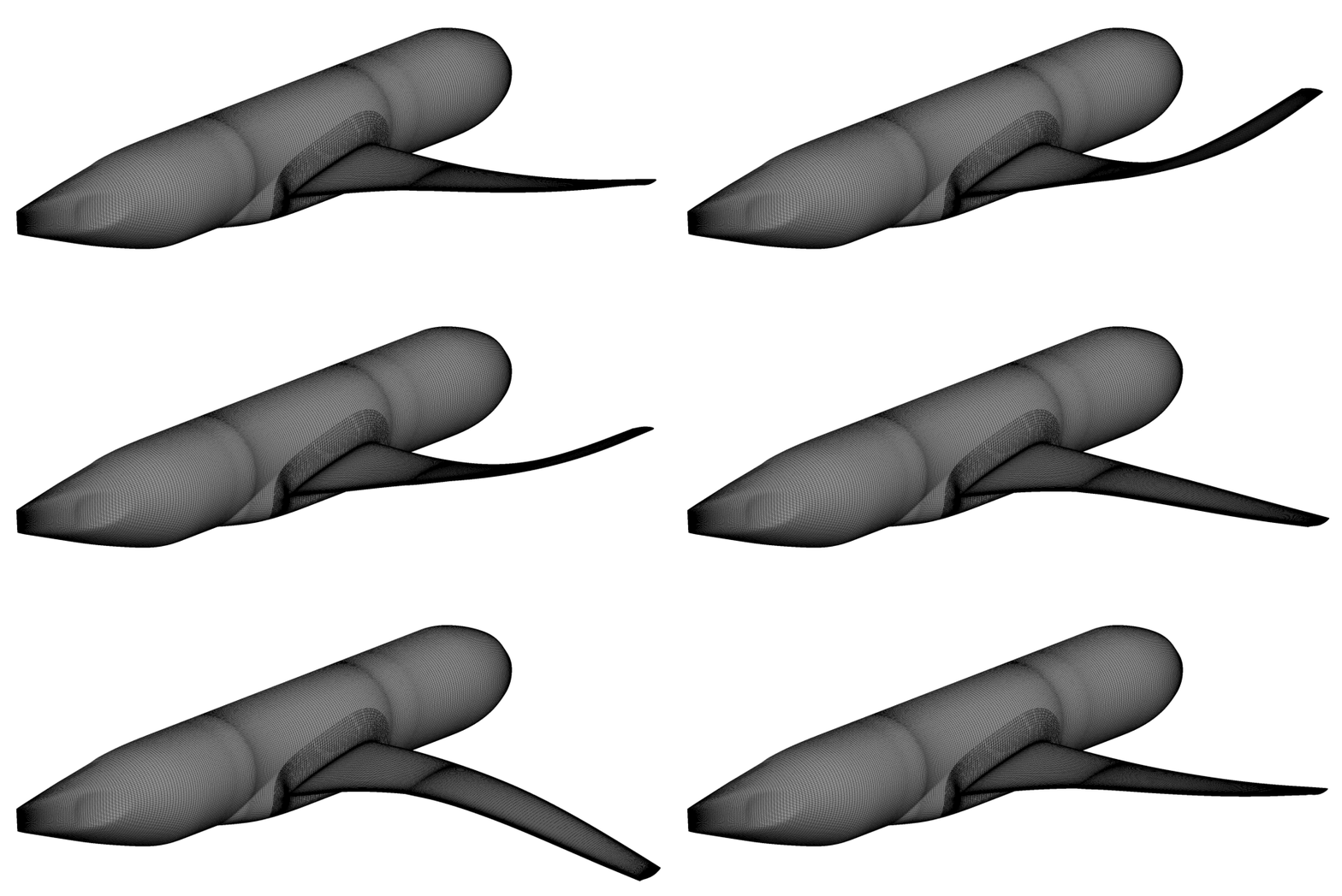
This tutorial demonstrates how to use LAVA's grid deformation capabilities to deflect the CRM wing to conform to a known bending and twist distribution. Specifically, we will be deflecting the wing to a prescribed bending and twist distribution corresponding to wind tunnel deflections at a 2.5 degree angle of attack.
Note that currently the figures in this tutorial do not contain the tail as they were re-appropriated from a prior optimization, but the tail is included here in the discussed files and tutorial process.
We will be leveraging LAVA's spline capabilities to create three B-Spline curves:
- a curve which follows the elastic axis inside the wing,
- a curve which interpolates the bending data at the sampled spanwise locations,
- a curve which interpolates the twist data at the sampled spanwise locations.
Rigid links will be created from each wing surface node to the elastic axis curve. These links are restricted to a constant \(y\) value, giving us a unique location along the elastic axis for each surface node. The bending and twist curves will then be used to define the desired deflection of the elastic axis, which will be applied to the wing surface nodes through a rotation and translation of the rigid links. Once we have obtained a deformed surface grid, we will use LAVA's grid deformation capabilities to deform the volume grid to conform to the new surface grid.
Case Setup
As a starting point, create a run sub-directory and generate a grid within
using run_buildGrid.sh as is done in the scripting
tutorial, or simply use the directory already
created for that tutorial. If you cannot or do not want to run that tutorial or
grid build script, the grid files relevant to this tutorial
(grid.x,grid.sur, and grid.bc) can be downloaded directly from the
scripting tutorial.
Run the init_morphing.sh script, within your chosen/created run sub-directory
(shown below). This creates a morphing sub-directory based on the (in this
case) angle of attack desired to be morphed to, then copies in the relevant
grid files along with the LAVA_morphing_ea.txt (elastic axis data),
LAVA_morphing_disp_aoa2p5.txt (bend/twist data), and LAVA_morphing.py (the
main morphing script) files needed to perform the morphing. Note that relevant
environmental variables and paths in the LAVA_morphing.py file are altered
according to the envVars.sh file entries, so ensure they are correct.
# Make a directory for the grid to have its wing morphed to 2.5 aoa position,
# copy in init grids and morping files, altering appropriately.
# This is set up to support a variety of AOA morphing cases, but each will need
# their own disp file, and only aoa 2.5 is supplied in the tutorial.
# ---------------------------------------------------------------------------- #
aoaOnes=(2)
aoaDecs=(5)

baseDir=$( cd -- "$( dirname -- "${BASH_SOURCE[0]}" )" &> /dev/null && pwd )

source $baseDir/envVars.sh

for ((aoaI=0; aoaI<${#aoaOnes[@]}; aoaI++)); do
    morphFolder="morphedGrid_aoa${aoaOnes[$aoaI]}p${aoaDecs[$aoaI]}"
    dispFile="LAVA_morphing_disp_aoa${aoaOnes[$aoaI]}p${aoaDecs[$aoaI]}.txt"
    jobPrefix="LAVA_morphing_aoa${aoaOnes[$aoaI]}p${aoaDecs[$aoaI]}"

    mkdir -p $morphFolder
    cd       $morphFolder

    cp                ../grid.x                        grid.in.x
    cp                ../grid.sur                      grid.in.sur
    cp                ../grid.bc                       grid.bc
    cp $baseDir/auxFiles/LAVA_morphing.py              .
    cp $baseDir/auxFiles/$dispFile                     .
    cp $baseDir/auxFiles/LAVA_morphing_ea.txt          .
    cp $baseDir/auxFiles/LAVA_morphing_rom_ait.pbs     .
    cp $baseDir/auxFiles/LAVA_morphing_tur_ath.pbs     .

    sed -i "/lava_suffix =/c\\lava_suffix = '$LAVA_EXE_SUFFIX'" \
           LAVA_morphing.py
    sed -i "/lava_lib_path =/c\\lava_lib_path = '$LAVA_LIB_DNY'" \
           LAVA_morphing.py
    sed -i "/disp_file =/c\\disp_file = \"$dispFile\"" \
           LAVA_morphing.py
    sed -i "#PBS -N/c\\#PBS -N ${jobPrefix}_rom_ait" \
           LAVA_morphing_rom_ait.pbs
    sed -i "/source path/c\\source $PY_VIRTUALENV_DIR" \
           LAVA_morphing_rom_ait.pbs
    sed -i "#PBS -W/c\\#PBS -W group_list=$GROUP_ID" \
           LAVA_morphing_rom_ait.pbs
    sed -i "#PBS -N/c\\#PBS -N ${jobPrefix}_tur_ath" \
           LAVA_morphing_tur_ath.pbs
    sed -i "/source path/c\\source $PY_VIRTUALENV_DIR" \
           LAVA_morphing_tur_ath.pbs
    sed -i "#PBS -W/c\\#PBS -W group_list=$GROUP_ID" \
           LAVA_morphing_tur_ath.pbs
done
# --------------------------------------------------------------------------- #
Running
Running on the NAS Cluster
You can run the morphing either locally or on the NAS cluster. The
init_morphing.sh script will have created two example pbs scripts for use on
NAS. If you aren't running all the tutorials on NAS, push the entire morphed_*
sub grid to nas to run.
Note that these pbs scripts will modify the LAVA_morphing.py file to have the
appropriate lava_suffix value once the job submits.
The charge group IDs of the pbs scripts, as well as the path to the Python
virtual environment you need to have set up on NAS should have been filled with
the variables you have set in envVars.sh file.
Running on External Systems
To run the morphing locally, navigate to the folder created by
init_morphing.sh, and run the run_morphing.sh script shown below. This
takes roughly 15 minutes with 1 MPI rank with 55 threads.
# Assumes init_morphing.sh has been called and you are running this on local
# compute from a directory created by it.
# ---------------------------------------------------------------------------- #
baseDir=$( cd -- "$( dirname -- "${BASH_SOURCE[0]}" )" &> /dev/null && pwd )

source $baseDir/envVars.sh

# Activate the python virtual environment.
source $PY_VIRTUALENV_DIR

# Set the LAVA lib suffix to the value within envVars.sh
sed -i "/lava_suffix =/c\\lava_suffix = '$LAVA_EXE_SUFFIX'" \
       LAVA_morphing.py

# Do the morphing (omp threads set in envVars.sh).
python LAVA_morphing.py | tee LAVA_morphing.out
# --------------------------------------------------------------------------- #
MPI Considerations
Warning
The LAVA_morphing.py script is not designed to run in parallel using MPI.
However, the LAVA dynamic libraries are generally compiled with both MPI
support and OpenMP thread support. Notably, the most computationally heavy
portion of the script is the volume mesh warping, which is performed by the
LAVA dynamic library. As such, the current tutorial will run in parallel
using OpenMP threads, but not MPI ranks. To extend this tutorial to MPI
ranks, you will need to partition the volume grid array vol_xyz across
MPI ranks and instantiate the meshWarper object on each rank with its
local portion of the volume grid. After warping is complete, you will then
need to gather the partitioned volume grid array back onto the root
processor for writing.
Morphing Python Script
This tutorial provides a single Python script, LAVA_morphing.py, which reads
in the elastic axis and displacement data, fits B-Spline curves to them, and
uses those curves to deflect the wing surface and volume grids. We will break
down the contents of this script below.
Imports
import numpy as np
import copy
from pylava.pyLAVA_spline import Curve
from pylava.pyLAVA_ioutils import (
    readPlot3DGrid,
    writePlot3DGrid,
    getPlot3DSurfaceConnectivity,
    collapseGrid,
    uncollapseGrid
)
from pylava.pyLAVA_meshwarp import meshWarper
Here, we import numpy and the standard library copy module, along with
three pieces of pyLAVA:
- the
Curveclass frompylava.pyLAVA_spline, which is used to create and evaluate B-Spline curves, - a collection of Plot3D grid I/O utilities from
pylava.pyLAVA_ioutils, and - the
meshWarperclass frompylava.pyLAVA_meshwarp, which is used to deform the volume grid.
Inputs
# Set the LAVA library name and path
lava_suffix = '3D.NS1.INTEL.AVX2.HPEMPT-lib'
lava_lib_path = None # If None, Python will search your LD_LIBRARY_PATH for the LAVA Dyn

# Input files
disp_file = "LAVA_morphing_disp_aoa2p5.txt"
ea_file = "LAVA_morphing_ea.txt"
surface_file = "grid.in.sur"
vol_file = "grid.in.x"

# Output files
surf_output_file = "grid.sur"
vol_output_file = "grid.x"

# Symmetry plane
symm_pts = [[0.0, 0.0, 0.0]]
symm_norms = [[0.0, 1.0, 0.0]]

# Span direction
span_dir = [0.0, 1.0, 0.0]

# List of surface blocks that define the wing
surf_deflect_block_list = list(range(4, 21))

# List of volume blocks to warp
vol_block_list = list(range(22))
print(f"Will be warping blocks {vol_block_list}", flush=True)
This section defines all of the inputs to the script:
lava_suffixandlava_lib_path: Tell pyLAVA which compiled LAVA dynamic library to use. Both theCurveandmeshWarperclasses below load this library directly. These entries should be automatically set by the init script above and by the pbs you run with: you should not have to set them in this file.disp_file: The text file containing the spanwise bending and twist distribution. Set by the init script above.ea_file: The text file containing the coordinates of the wing's elastic axis.surface_fileandvol_file: The undeformed surface and volume grid files.surf_output_fileandvol_output_file: The names of the deflected surface and volume grid files that will be written out by this script.symm_ptsandsymm_norms: A point and normal vector defining the symmetry plane, used by the mesh warper.span_dir: The direction of the wing span, used to define the axis about which the wing will twist.surf_deflect_block_list: The list of surface grid zones that make up the wing; only these zones will be deflected.vol_block_list: The list of volume grid zones that will be warped to conform to the deflected surface.
Note
The ea_file and disp_file inputs are expected to be sampled at the same
spanwise stations, i.e., they must contain the same number of rows in the
same order. This is because the parametric locations along the elastic axis
curve, computed from ea_file, are reused directly to fit the bending and
twist curves from disp_file below.
If you want to run extra aoa displacements, you must both supply those
appropriately named extra disp files and add them to the auxFiles folder,
and then update the init_morphing.sh file to include the new aoa numbers.
Helper Function
def compute_surf(surf_pts_0, link_s, ea_curve, bend_curve, rot_curve):
    """Deflect the wing surface based on bending and rotation curves.

    Args:
        surf_pts_0: Original surface points
        link_s: Parametric locations along the elastic axis
        ea_curve: Elastic axis curve
        bend_curve: Bending displacement curve
        rot_curve: Rotation (twist) curve

    Returns:
        surf_pts: Deflected surface points
    """
    surf_pts = np.zeros_like(surf_pts_0)

    # Rotate and displace each surface point
    for i in range(surf_pts_0.shape[0]):
        # Parametric location on curve
        s = link_s[i]

        # Point on elastic axis curve
        curveXYZ = ea_curve(s)

        # Link vector from curve to surface point
        linkVec = surf_pts_0[i, :] - curveXYZ

        # Rotation angle (convert to radians)
        ang = rot_curve(s) * np.pi / 180.0

        # Create rotation matrix (rotation about y-axis)
        Ry = np.array([
            [np.cos(ang), 0.0, np.sin(ang)],
            [0.0, 1.0, 0.0],
            [-np.sin(ang), 0.0, np.cos(ang)]
        ])

        # Rotate the link vector
        linkVec = np.dot(Ry, linkVec)

        # Apply rotation and bending displacement
        surf_pts[i, :] = curveXYZ + linkVec
        surf_pts[i, 2] += bend_curve(s)

    return surf_pts
The compute_surf function computes the deflected location of a single set of
surface points, given their parametric locations (link_s) along the elastic
axis curve. For each surface point:
- The corresponding point on the elastic axis curve is evaluated at the
point's parametric location,
s. - A rigid link vector is formed between this point on the elastic axis and the original (undeflected) surface point.
- The twist curve is evaluated at
sto get the local twist angle, which is used to build a rotation matrix about the span direction (the \(y\)-axis, in this example). - The link vector is rotated by this rotation matrix.
- The deflected surface point is obtained by adding the rotated link vector to
the point on the elastic axis, then adding the local bending displacement
(evaluated from the bending curve at
s).
To demonstrate this, we first visualize a rigid link (shown in red) between a single surface point and the elastic axis (shown in blue).
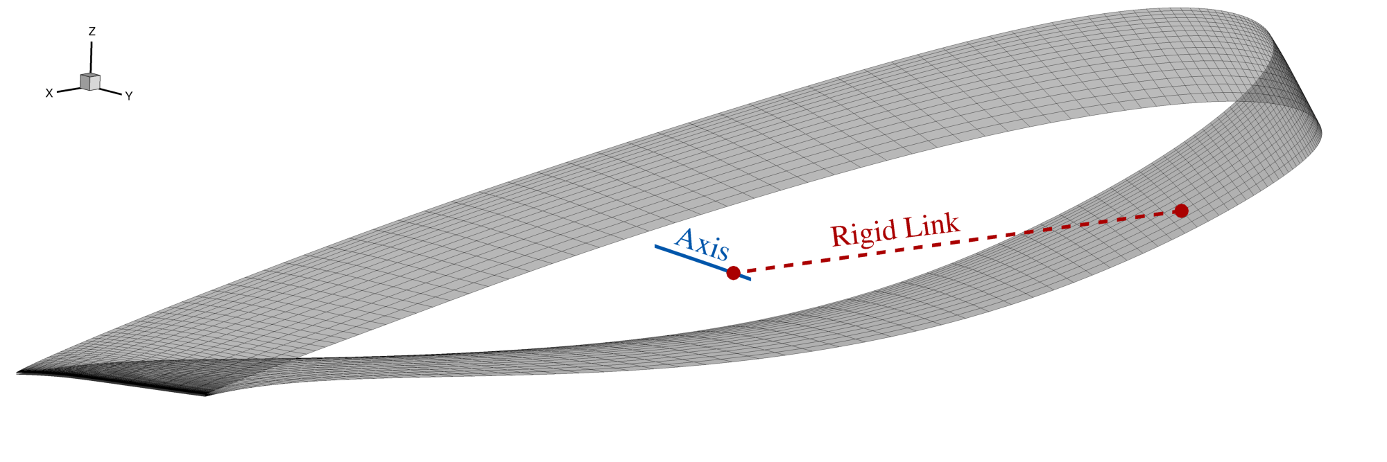
The wing can be rotated by simply rotating each rigid link about the elastic axis. Similarly, translation can be applied to the wing by translating each rigid link. In the following figure, we demonstrate the application of a rotation about the elastic axis.
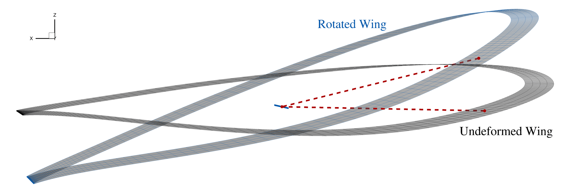
As previously mentioned, local bending (translation) and twist (rotation) values are obtained from the bending and twist curves.
Creating the Elastic Axis Curve
# Read and create the elastic axis curve
ea = np.loadtxt(ea_file, skiprows=1)[:, 1:].copy()
ea_curve = Curve(lava_suffix, lava_lib_path, X=ea)
ea_curve.writeTecplot("ea_curve.dat")

# Get arc length parameterization for the original data
s = ea_curve.getOrigDataParameterization()
Here, we read in the \((x,y,z)\) coordinates of the elastic axis from ea_file
and create a Curve object, ea_curve, which locally interpolates these
points. The curve is written out to a Tecplot file, ea_curve.dat, so that it
can be visualized alongside the grid, as in the following image.
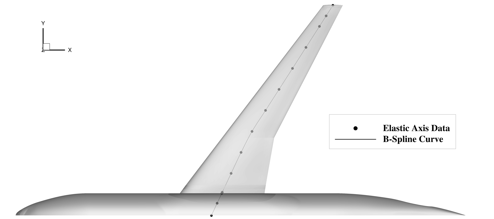
We then call getOrigDataParameterization to retrieve the parametric location,
s, of each of the original elastic axis data points along the curve. These
parametric locations will be reused below to fit the bending and twist curves
at the same spanwise stations.
Fitting the Bending and Twist Curves
# Read and fit the bending displacement data
bend_data = np.loadtxt(disp_file, skiprows=1)[:, 1].copy()
bend_curve = Curve(lava_suffix, lava_lib_path, X=bend_data, s=s, k=4, nIter=100)

err = np.linalg.norm(bend_data - bend_curve(s))
print(f"Displacement Fitting Error: {err}")
# Read and fit the twist data
twist_data = np.loadtxt(disp_file, skiprows=1)[:, 2].copy()
twist_curve = Curve(lava_suffix, lava_lib_path, X=twist_data, s=s, k=4, nIter=100)

err = np.linalg.norm(twist_data - twist_curve(s))
print(f"Twist Fitting Error: {err}")
Next, we read in the bending and twist data from disp_file and fit a B-Spline
curve to each using a least-mean-squares fit (k=4, nIter=100), evaluated at
the same parametric locations, s, as the elastic axis curve. The fitting
error, the \(L_2\) norm between the raw data and the curve evaluated at s, is
printed to the screen so that you can confirm the curve is an adequate fit to
your data.
The figure below demonstrates the B-Spline fit of the bending and twist data,
along with the original data points. 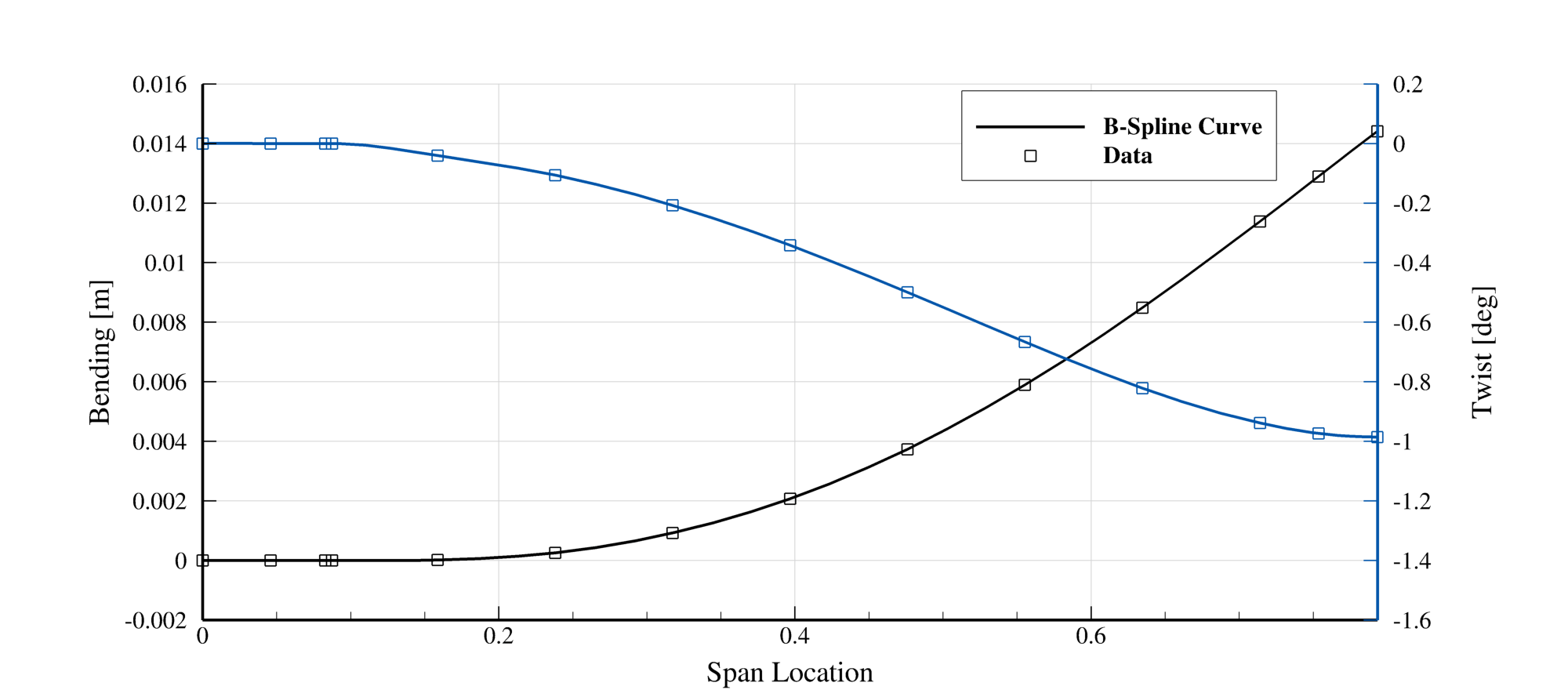
Reading and Selecting the Wing Surface Grid
# Read the surface grid
surf_nzones, surf_sizes, surf_zones = readPlot3DGrid(
    surface_file, hasRM=True, hasIB=False
)
conn = getPlot3DSurfaceConnectivity(surf_sizes)
surf_xyz_0, _, surf_conn = collapseGrid(
    surf_nzones, surf_sizes, surf_zones, conn=conn
)
# Extract the wing surface blocks to deform
select_surf_zones = [surf_zones[i] for i in surf_deflect_block_list]
select_surf_sizes = np.asarray([surf_sizes[i] for i in surf_deflect_block_list])
select_surf_xyz_0, _ = collapseGrid(
    len(select_surf_zones), select_surf_sizes, select_surf_zones
)
We read in the full surface grid, grid.sur, and use
getPlot3DSurfaceConnectivity and collapseGrid to build a single array of
unique surface points and their connectivity, surf_xyz_0 and surf_conn.
This representation is required later by the meshWarper. From this full
surface, we then extract just the zones that make up the wing, as specified by
surf_deflect_block_list, and collapse them into their own array,
select_surf_xyz_0. Only these points will be deflected.
Deflecting the Wing Surface
# Create rigid links and compute displaced surface
link_s, _ = ea_curve.intersectPlane(select_surf_xyz_0, np.array(span_dir))
select_surf_xyz = compute_surf(
    select_surf_xyz_0, link_s, ea_curve, bend_curve, twist_curve
)

# Reconstruct the surface zones
new_select_surf_zones = uncollapseGrid(
    len(select_surf_zones), select_surf_sizes, select_surf_xyz
)

# Update the full surface with deflected wing blocks
new_surf_zones = copy.deepcopy(surf_zones)
for i, new_surf_zone in zip(surf_deflect_block_list, new_select_surf_zones):
    new_surf_zones[i] = new_surf_zone

# Write the deflected surface
writePlot3DGrid(surf_output_file, new_surf_zones)

# Collapse the new surface for warping
surf_xyz, _ = collapseGrid(surf_nzones, surf_sizes, new_surf_zones)
For each wing surface point, we call intersectPlane on the elastic axis curve
to find the parametric location, link_s, of the plane (normal to span_dir)
that passes through that point and intersects the elastic axis curve. This
defines the rigid link between each surface point and the elastic axis. The
compute_surf helper function (discussed above) is then used to compute the
deflected wing surface points, select_surf_xyz, from these links and the
bending and twist curves. The deflected wing zones are reconstructed with
uncollapseGrid, and swapped into a copy of the full surface grid in place of
the original wing zones. This new surface grid is written out to
surf_output_file and collapsed again for use in the volume warp below.
Warping the Volume Grid
# Read and prepare the volume grid
vol_nzone, vol_sizes, vol_zones = readPlot3DGrid(
    vol_file, hasRM=True, hasIB=False
)

select_zones = [vol_zones[i] for i in vol_block_list]
select_sizes = np.asarray([vol_sizes[i] for i in vol_block_list])
vol_xyz, _ = collapseGrid(len(select_zones), select_sizes, select_zones)

# Initialize the mesh warper
warper = meshWarper(
    surf_xyz_0,             # Original surface coordinates
    surf_conn,              # Surface connectivity
    vol_xyz,                # Volume coordinates
    symm_pts=symm_pts,      # Symmetry plane points
    symm_norms=symm_norms,  # Symmetry plane normals
    suffix=lava_suffix,     # LAVA DLL suffix
    libPath=lava_lib_path,  # LAVA DLL path
    warp_options={},
)

# Warp the volume grid
new_vol_xyz = warper.warpMesh(surf_xyz)

# Reconstruct volume zones
new_vol_zones = uncollapseGrid(len(select_zones), select_sizes, new_vol_xyz)

# Update the full volume grid with warped blocks
for i, new_vol_zone in zip(vol_block_list, new_vol_zones):
    vol_zones[i] = new_vol_zone

# Write the warped volume grid
writePlot3DGrid(vol_output_file, vol_zones)
Finally, we read in the volume grid, grid.x, and collapse the blocks to be
warped, as specified by vol_block_list, into a single array of points,
vol_xyz. We then instantiate the meshWarper object, giving it the
original (undeflected) surface points and connectivity, the volume points to
be warped, and the symmetry plane definition. A call to warper.warpMesh,
passing in the deflected surface coordinates, propagates the surface
deflection through the volume grid using LAVA's mesh warping algorithm. The
warped volume grid blocks are reconstructed with uncollapseGrid, swapped into
the full set of volume zones, and written out to vol_output_file.
Post-Processing
Running LAVA_morphing.py produces three output files:
surf_output_file(grid.2_50.surin this example) : The deflected surface grid, in Plot3D format.vol_output_file(grid.2_50.xin this example) : The volume grid, warped to conform to the deflected surface.ea_curve.dat: A Tecplot file containing the fitted elastic axis curve, along with its control points and the original elastic axis data.
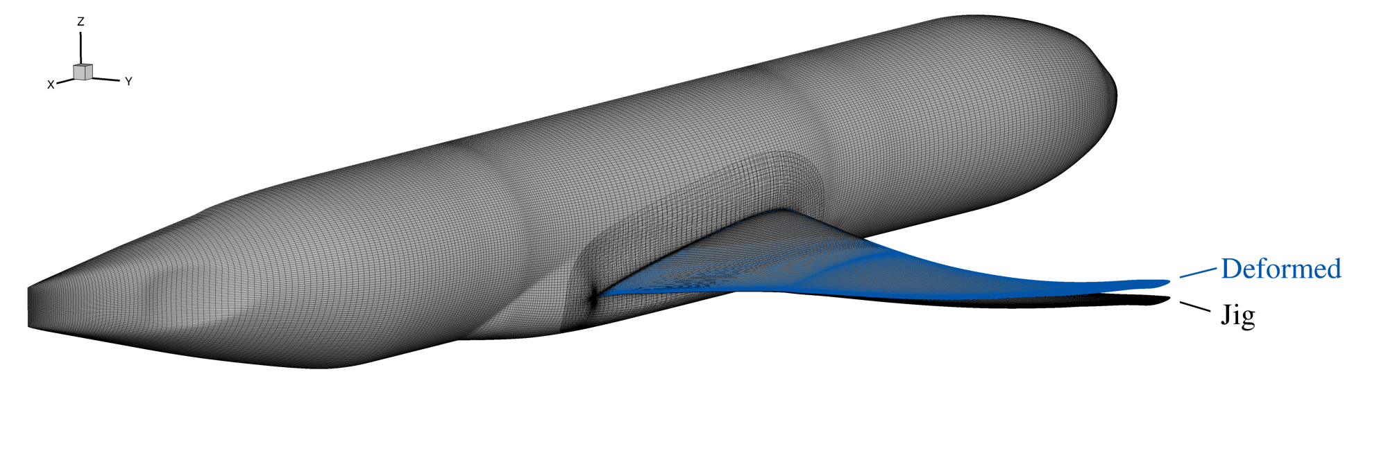
The undeformed and deflected surface and volume grids can be viewed together in
Tecplot, or any other visualization software that supports the Plot3D format,
in conjunction with grid.x. The bending and twist fitting errors printed to
the screen during the run should also be checked to confirm that the fitted
curves are an adequate representation of your input displacement data.
Solution Pre-processing
Prior to performing solutions on the newly deformed grid, run the
run_connectivity.sh script or run on NAS as described in the connectivity
tutorial: no changes need to be made to
the connectivity files themselves because the grid files are named as expected.