Performing Design Optimization
This tutorial demonstrates how to set up and use gradient‑based design optimization with the LAVA Curvilinear solver to minimize the drag on the CRM while meeting target lift and pitching moment requirements. The optimization is performed using OpenMDAO1 and MPhys2.
We will be replicating the 5th test case from the suite provided by the AIAA Aerodynamic Design Optimization Discussion Group, though at a lower Reynolds number. Specifically, at Mach of 0.85 and Re of 5 million, we solve the following optimization problem:
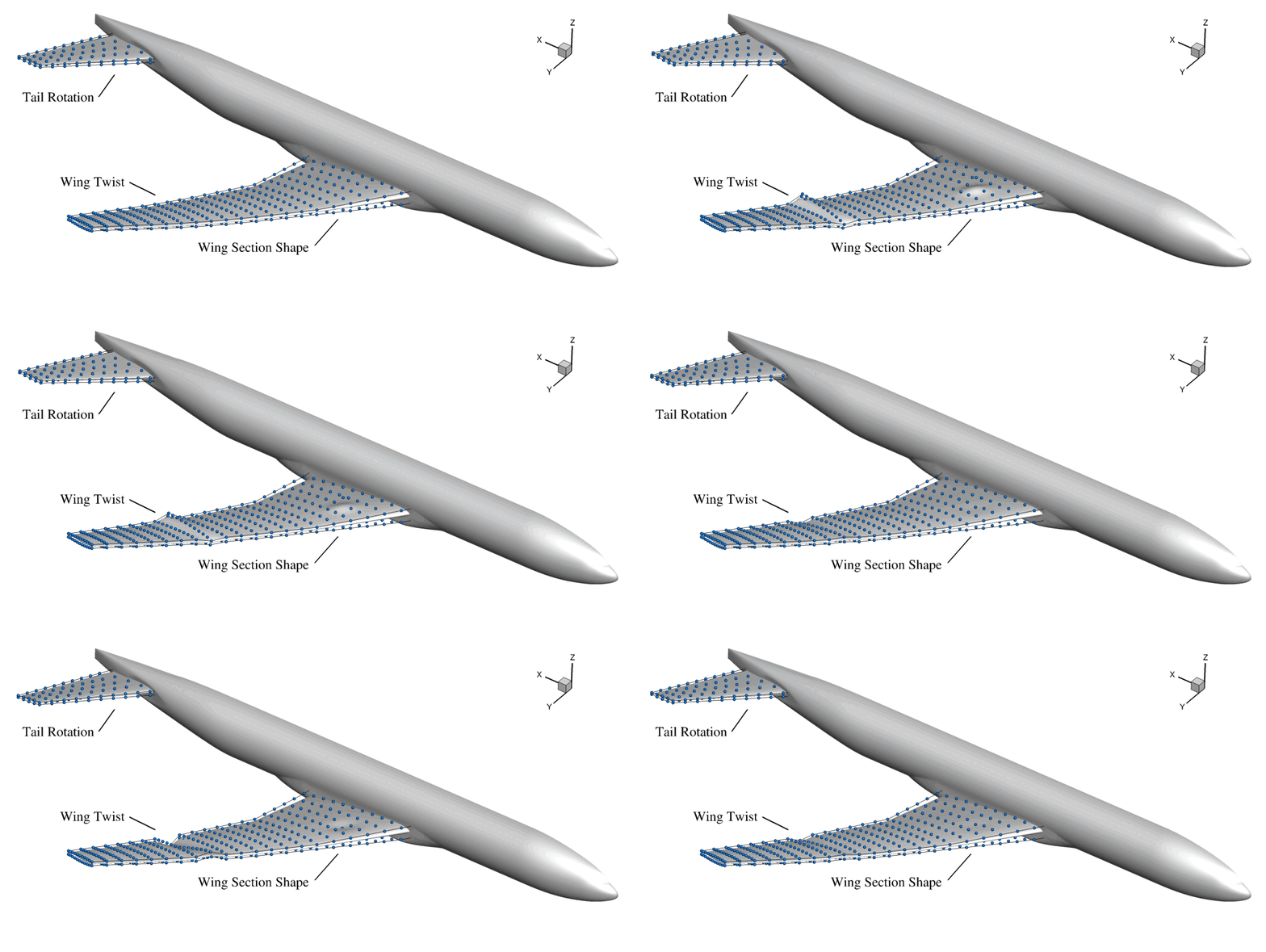
The geometric design variables are visualized below:
The box below demonstrates the N2 diagram for the OpenMDAO model constructed in
this tutorial. It is interactive, so you can click on the components to see
their inputs and outputs. The entire cruise group in the model consists of
different parts of the LAVA Curvilinear framework. The aero_pre component is
LAVA's volume mesh warper which takes in a surface mesh and outputs a deformed
volume mesh. The solver component contains both the LAVA Curvilinear flow
solver and the discrete adjoint solver; it takes the volume grid coordinates
and the angle of attack as inputs, and outputs the flow state vector. The
aero_post component is LAVA's functional computation capability, which takes
in the flow field states, the volume grid coordinates, and the angle of attack,
and outputs the aerodynamic functionals of interest.
Warning
The optimization features in LAVA are still evolving, and you may encounter bugs or unexpected behavior. The steps in and results from this tutorial have been tested and are expected to work as described.
Case Setup
As a starting point, create a run sub-directory and generate a grid within
using run_buildGrid.sh as is done in the scripting
tutorial, then connect it as is done in the
connectivity tutorial, or simply use the
directory already created for those tutorials. If you cannot or do not want to
run that tutorial or grid build script, the grid files relevant to this
tutorial (grid.x.ihc, grid.bc, grid.x.b2b, panel_weights.dat (place
into overlapper sub folder), and INTOUT) can be downloaded directly from
those tutorials.
Run the init_design.sh script, within your chosen/created run sub-directory
(shown below). This creates a design sub-directory based on the components you
desire to design, then copies in the relevant python, yaml and pbs files along
with the component surface triangualations which associate grid movement, and
FFDs which control that movement. Note that relevant environmental variables
and paths in the LAVA_design.py file are altered according to the
envVars.sh file entries, so ensure they are correct. For organization, ffds
and triSurfs sub folders are created.
# Takes a list of components (comps, first line below), and makes an
# appropriate subdirectory to perform the design optimization. A design file
# tree is created and all needed files are copied in, altered if need be.
#
# Currently, the MDAO-based LAVA_design_*.py file is too granularly hard-coded
# to allow for proper comp scripting, so for now if you want to make a new
# design, you must make a new LAVA_design_*.py file in auxFiles appropriately
# named for the components. All other files need not be changed (though some
# triSurfs and ffds may need to be added).
#
# For this tutorial, only the fuse, wing, and tail together are considered.
# --------------------------------------------------------------------------- #
comps=(fuse wing tail)

compList="${comps[*]}"
comp_list=$(IFS=_; echo "${comps[*]}")
compComlist=$(IFS=, ; echo "${comps[*]}")

baseDir=$( cd -- "$( dirname -- "${BASH_SOURCE[0]}" )" &> /dev/null && pwd )

source $baseDir/envVars.sh

mkdir -p design_${comp_list}
cd       design_${comp_list}
mkdir -p ffds
mkdir -p triSurfs

cp $baseDir/auxFiles/LAVA_design_${comp_list}.py LAVA_design.py
cp $baseDir/auxFiles/LAVA_design_postProc.py .
cp $baseDir/auxFiles/LAVA_solver_design.yaml .
cp $baseDir/auxFiles/LAVA_design_tur_ath.pbs .
cp $baseDir/auxFiles/LAVA_design_rom_ait.pbs .

sed -i "/my_lava_suffix =/c\\my_lava_suffix='$LAVA_EXE_SUFFIX'" \
       LAVA_design.py

sed -i "/wallCompNamesHere/c\\    names : [$compComlist]" \
       LAVA_solver_design.yaml

sed -i "/#PBS -N/c\\#PBS -N LAVA_design_${comp_list}_rom_ait" \
       LAVA_design_tur_ath.pbs
sed -i "/source path/c\\source $PY_VIRTUALENV_DIR" \
       LAVA_design_tur_ath.pbs
sed -i "/#PBS -W/c\\#PBS -W group_list=$GROUP_ID" \
       LAVA_design_tur_ath.pbs
sed -i "s/pythonX.XX/python$PYTHON_VERSION/g" \
       LAVA_design_tur_ath.pbs

sed -i "/#PBS -N/c\\#PBS -N LAVA_design_${comp_list}_tur_ath" \
       LAVA_design_tur_ath.pbs
sed -i "/source path/c\\source $PY_VIRTUALENV_DIR" \
       LAVA_design_tur_ath.pbs
sed -i "/#PBS -W/c\\#PBS -W group_list=$GROUP_ID" \
       LAVA_design_tur_ath.pbs

for ((compI=0; compI<${#comps[@]}; compI++)); do
    comp="${comps[$compI]}"
    compCapps=$(echo "$comp" | tr '[:lower:]' '[:upper:]')

    cp $baseDir/geom/$comp/${compCapps}_TRISURF.*    triSurfs/
    cp $baseDir/auxFiles/LAVA_design_FFD_${comp}.xyz ffds/
done

cd triSurfs

for file in *zip*; do
    unzip -q -o $file
done
# --------------------------------------------------------------------------- #
Running
Currently, this tutorial utilizes the nonlinear optimizer
SNOPT, with the Python
interface provided by
pyOptSparse3. You may try
your hand at using alternative optimizers for this problem, though your mileage
may vary. pySurf is used to deform
junctions.
Running on the NAS Cluster
You can run the design either locally or on the NAS cluster. The
init_design.sh script will have created two pbs scripts for use on NAS. If
you aren't running all the tutorials on NAS, push the entire design_* sub
directory to nas to run.
Note that the pbs script will modify the LAVA_design.py file to have the
appropriate my_lava_suffix value once the job submits.
The charge group IDs of the pbs scripts, as well as the path to the Python
virtual environment you need to have set up on NAS should have been filled with
the variables you have set in envVars.sh file.
If running on 8 Athena nodes, the design process takes roughly 56 hours for the required 270 function evaluations.
Running on External Systems
To run the design locally (not recommended due to resource requirements),
navigate to the folder created by init_design.sh, and run the run_design.sh
script shown below.
# Assumes init_design.sh has been called and you are running this on local
# compute from a directory created by it.
# ---------------------------------------------------------------------------- #
baseDir=$( cd -- "$( dirname -- "${BASH_SOURCE[0]}" )" &> /dev/null && pwd )

source $baseDir/envVars.sh

# Activate the python virtual environment.
source $PY_VIRTUALENV_DIR

# Set the LAVA lib suffix to the value within envVars.sh
sed -i "/my_lava_suffix =/c\\my_lava_suffix = '$LAVA_EXE_SUFFIX'" \
       LAVA_design.py

# Do the design (omp threads set in envVars.sh).
if (( N_PROC > 1 )); then
    mpiproc -np $N_PROC python LAVA_design.py | tee LAVA_design.out
else
    python LAVA_design.py | tee LAVA_design.out
fi
# --------------------------------------------------------------------------- #
Python Script
The main script of this tutorial is the LAVA_design.py Python script that
will have been copied into the created design sub directory, which is
responsible for running the optimization problem using OpenMDAO, MPhys, and
pyLAVA. When the init script is run, it copies in the appropriate design python
script from auxFiles according to the components you requested and renames it
sans components. We will break down the contents of this script below, which is
the example given if the fuse, wing, and tail all were to be considered
(LAVA_design_fuse_wing_tail.py). As things are currently set up, you would
have to make a new LAVA_design_*.py file for a different component set.
Imports
import openmdao.api as om
from mphys import MPhysVariables, Multipoint
from mphys.scenarios.aerodynamic import ScenarioAerodynamic
from pylava.mphys.mphys_lava import LAVABuilder
from pygeo.mphys import OM_DVGEOCOMP
from pyspline import Curve
In the imports section, we import the necessary modules from OpenMDAO, MPhys,
pyLAVA, pyGeo, and pySpline. This includes the LAVABuilder class from
pylava.mphys.mphys_lava, which is used to create the LAVA flow solver
component for MPhys.
Read YAML
        # Read the YAML file for lava options
        with open("LAVA_solver_design.yaml", "r") as f:
            lava_options = yaml.safe_load(f)
Here, we load the YAML configuration file into a Python dictionary. The
lava.yaml file contains all the input parameters for the LAVA flow solver.
LAVA MPhys Builder
        # LAVA Builder
        lava_builder = LAVABuilder(lava_options, scenario="aerodynamic",
                                   lava_suffix=my_lava_suffix,
                                   design_surf_fams=["wing", "fuse", "tail"],
                                   functionals=["cl", "cd", "cmy"])
        lava_builder.initialize(self.comm)
MPhys leverages
builders to create the
necessary components for a multidisciplinary analysis and optimization. When
instantiating the LAVABuilder, several arguments can be passed. In this
tutorial we pass the following:
lava_options: The dictionary of options for the LAVA flow and adjoint solvers, loaded fromlava.yamlabove.scenario: The MPhys scenario to be used. We use"aerodynamic"for aerodynamic analysis.lava_suffix: Specifies which compiled LAVA dynamic library to use. This must match the LAVA installation on your system.design_surf_fams: A list of surface family names that will be used for geometric design variables. In this case, we use thewing,fuse, andtailsurface families. Note that these families are specified in thegrid.bcboundary condition file.functionals: These are the aerodynamic functionals that will be set as outputs to the LAVA OpenMDAO Group, making them available for use as objectives or constraints. In this case, we usecl,cd, andcmy(lift, drag, and pitching moment coefficients).
Since the optimization problem minimizes drag subject to lift and pitching
moment constraints, cd serves as the objective, while cl and cmy are
constraints.
MPhys Setup
        # == MPhys Setup ==

        # Keep DVs at the top level
        self.add_subsystem('dvs', om.IndepVarComp(), promotes=['*'])

        # Add mesh to subsystems
        self.add_subsystem('mesh', lava_builder.get_mesh_coordinate_subsystem())

        # Add the geometry component from pyGeo (multi-component FFD)
        self.add_subsystem('geometry', OM_DVGEOCOMP(type='multi'))

        # We're cruisin
        self.mphys_add_scenario('cruise', ScenarioAerodynamic(aero_builder=lava_builder))

        # Ensure that the mesh and cruise coordinates are the same
        self.connect(
            f"mesh.{MPhysVariables.Aerodynamics.Surface.Mesh.COORDINATES}",
            f"geometry.{MPhysVariables.Aerodynamics.Surface.Geometry.COORDINATES_INPUT}")
        self.connect(
            f"geometry.{MPhysVariables.Aerodynamics.Surface.Geometry.COORDINATES_OUTPUT}",
            f"cruise.x_aero")
In the MPhys setup portion of the Multipoint OpenMDAO Group, several steps occur:
- An independent variable component
dvsis added to hold the design variables for the optimization problem. - A component
meshis added to output the undeformed surface mesh from the LAVA solver. - A
geometrycomponent is added using pyGeo'sOM_DVGEOCOMP, which handles the geometric design variables and deformation. - The scenario's
add_scenariomethod is called to add an aerodynamic scenario to the MPhys Group. - Connections are made between components: the undeformed surface mesh flows
from
meshtogeometry, and the deformed surface mesh flows fromgeometryto the aerodynamic scenario.
Most of this setup is standard for MPhys-based aerodynamic optimization problems, which is described in more detail in the MPhys documentation.
Geometry Parameterization
FFD Setup
        # == FFD Setup ==

        # Wing FFD
        self.geometry.nom_addComponent(
            comp="wing",
            ffd_file=os.path.join("ffds", "LAVA_design_FFD_wing.xyz"),
            triMesh=os.path.join("triSurfs", "WING_TRISURF.cgns")
        )

        # Fuselage and Vertical Tail FFD
        self.geometry.nom_addComponent(
            comp="fuse",
            ffd_file=os.path.join("ffds", "LAVA_design_FFD_fuse.xyz"),
            triMesh=os.path.join("triSurfs", "FUSE_TRISURF.cgns")
        )

        # Horizontal Tail FFD
        self.geometry.nom_addComponent(
            comp="tail",
            ffd_file=os.path.join("ffds", "LAVA_design_FFD_tail.xyz"),
            triMesh=os.path.join("triSurfs", "TAIL_TRISURF.cgns")
        )
The call to
nom_addComponent
of the OM_DVGEOCOMP object is used to add a component to the geometry setup.
See pyGeo's OM_DVGEOCOMP
documentation
for more information on this method. We add three components (wing, fuselage,
and tail), each with:
comp: The name of the component.ffd_file: The path to the Plot3D file containing the Free-Form Deformation (FFD) volume for this component. The FFD volume controls how the aerodynamic surface deforms when design variables are applied.triMesh: The path to the surface triangulation file (stored as a.cgnsfile) for this component. See the DVGeometryMulti documentation for more information on this file.
Intersection Setup
        # == Intersection Setup ==
        # Note: Intersections must be defined before adding the pointset

        # Wing-Fuse Intersection
        DVGeoMulti.addIntersection(
            compA="fuse",
            compB="wing",
            dStarA=0.081,
            dStarB=0.005,
            featureCurves=["wing_LE_0_CURVE", "wing_TE_0_CURVE", "wing_TE_1_CURVE"],
            project=True,
            marchDir=2,
            includeCurves=True,
            curveEpsDict={
                'intersection': 1.e-4,
                'wing_LE_0_CURVE': 1.e-6,
                'wing_TE_0_CURVE': 8.e-6,
                'wing_TE_1_CURVE': 8.e-6,
            },
        )

        # Tail-Fuse Intersection
        DVGeoMulti.addIntersection(
            compA="fuse",
            compB="tail",
            dStarA=0.081,
            dStarB=0.027,
            featureCurves=["tail_LE_0_CURVE", "tail_TE_0_CURVE", "tail_TE_1_CURVE"],
            project=True,
            marchDir=2,
            includeCurves=True,
            curveEpsDict={
                'intersection': 1.e-2,
                'tail_LE_0_CURVE': 1.e-6,
                'tail_TE_0_CURVE': 4.e-6,
                'tail_TE_1_CURVE': 4.e-6,
            }
        )

        # NOTE: Because we are working with a 2.7% scale model of the CRM,
        # the default zero cutoff for the inverse distance weighted integral
        # is too large and must be reduced
        for intersections in DVGeoMulti.intersectComps:
            intersections.eps = 1.e-28
Intersections between components must be explicitly stated via a call to the
addIntersection
function of the DVGeometryMulti class. Here we specify two intersections:
- Wing-Fuselage Intersection: Where the wing meets the fuselage. The
parameters
dStarAanddStarBcontrol the blend distance on each component,featureCurvesspecifies important geometry features to preserve, andcurveEpsDictdefines tolerances for fitting these curves. - Tail-Fuselage Intersection: Where the horizontal tail meets the fuselage, with similar parameters to control the deformation at the junction.
These intersections ensure that when the wing or tail deforms, the fuselage surface smoothly blends with these deformations, maintaining surface continuity and proper aerodynamic shape.
Additionally, because we are working with a 2.7% scale model of the CRM, the
default inverse distance weighted integral cutoff (eps) must be reduced to
prevent numerical issues in the intersection handling.
Pointset Setup
        # == Pointset Setup ==
        # Add points from LAVA's design surface
        points = self.mesh.mphys_get_surface_mesh()
        self.geometry.nom_add_discipline_coords(
            MPhysVariables.Aerodynamics.Surface.Geometry,
            points, applyIC=True)
The pointset setup specifies the surface points that will be used for geometric
design variables and constraints. The call to
self.mesh.mphys_get_surface_mesh() retrieves the entire surface mesh from the
LAVA Curvilinear solver for all families previously specified in the
design_surf_fams argument of the LAVABuilder. When passing all surface
points to the OM_DVGEOCOMP component, it will automatically organize and sort
the points into the appropriate components for deformation.
Design Variables Setup
        # == Design Variable Setup ==

        # Wing Twist
        # Create a reference axis in the wing FFD
        nRefAxPts = self.geometry.nom_addRefAxis(name="wingaxis", xFraction=0.25,
                                                 alignIndex="j", comp="wing")
        nTwist = nRefAxPts

        # Setup the global twist DVs for the wing FFD
        def wingtwist(val, geo):
            for i in range(0, nRefAxPts):
                geo.rot_y["wingaxis"].coef[i] = val[i]
        self.geometry.nom_addGlobalDV(dvName="wingtwist", value=np.zeros((nTwist)),
                                      func=wingtwist, comp="wing")

        # Wing Shape
        # Setup the local section shape DVs for the wing FFD
        nLocal = self.geometry.nom_addLocalDV(dvName="wingshape", axis="z", comp="wing")

        # Tail Twist
        # Create a reference axis for the tail FFD
        xyz = np.array([[4.6750224, 0., 0.052832], [4.6750224, 0.3, 0.052832]])
        axialCurve = Curve(x=xyz[:, 0], y=xyz[:, 1], z=xyz[:, 2], k=4)
        nRefAxPts_tail = self.geometry.nom_addRefAxis(name="tailaxis", curve=axialCurve,
                                                      axis="x", comp="tail")
        nTwist_tail = nRefAxPts_tail

        # Setup the global twist DV for the tail FFD
        def tailtwist(val, geo):
            for i in range(0, nRefAxPts_tail):
                geo.rot_y["tailaxis"].coef[i] = val[0]
        self.geometry.nom_addGlobalDV(dvName="tailtwist", value=np.zeros((1)),
                                      func=tailtwist, comp="tail")
In this portion of the Python script, we define the geometric design variables for the optimization problem. These include:
- Wing Twist: A global twist design variable that rotates the wing about a
reference axis (at 25% chord). A reference axis is created using
nom_addRefAxis, and the global twist is applied at multiple spanwise locations. - Wing Section Shape: Local shape design variables that allow each wing section to deform in the vertical (z) direction, enabling changes to the wing's aerodynamic profile.
- Tail Angle: A global twist design variable for the tail that rotates about a specified axis. The axis is defined by a B-Spline curve created from two endpoints with the same (x, z) coordinates but spanning the full tail length in the y-direction.
Please refer to this OM_DVGEOCOMP documentation for more information on the available options for design variables.
Geometric Constraints
        # == Geometric Constraint Setup ==

        # Setup surface triangulation
        tri_file = os.path.join("triSurfs", "WING_TRISURF.tri")
        f = FortranFile(tri_file, 'r')

        # Read tri-file's vertice and connectivity info
        nVerts, nTri = f.read_ints()
        xyz = f.read_reals(dtype='f4').reshape((nVerts, 3))
        conn = f.read_ints().reshape((nTri, 3)) - 1
        tri_surf = np.zeros((nTri, 3, 3))
        for i in range(3):
            tri_surf[:, i, :] = xyz[conn[:, i], :]
        self.geometry.nom_setConstraintSurface(tri_surf, surfFormat="point-point")

        # Nonlinear thickness constraint
        leList = np.loadtxt(os.path.join("constraint", "LE.dat"), skiprows=1)
        teList = np.loadtxt(os.path.join("constraint", "TE.dat"), skiprows=1)
        self.geometry.nom_addThicknessConstraints2D("thickcon", leList, teList, nSpan=40,
                                                    nChord=30, projected=True,
                                                    compNames=['wing'])

        # Add fixed LE/TE constraints
        self.geometry.nom_add_LETEConstraint('tecon', 0, 'ihigh', comp='wing')
        self.geometry.nom_add_LETEConstraint('lecon', 0, 'ilow', comp='wing')
In this section, geometric constraints are applied to the wing to ensure that the optimized design meets physical requirements:
- Surface Triangulation: A surface triangulation file is read to represent the reference aerodynamic surface. This is used to define the constraint surface against which other constraints are measured.
- Thickness Constraints: Nonlinear constraints that ensure the wing maintains minimum thickness between leading and trailing edge points. These constraints are applied at 40 spanwise and 30 chordwise locations, and are projected onto the aerodynamic surface.
- Leading/Trailing Edge Constraints: Fixed constraints that prevent the leading and trailing edges of the wing from moving, maintaining the geometric definition of these important features.
These constraints work together to ensure the optimized design is physically realizable while meeting the aerodynamic objectives.
OpenMDAO Setup
        # == OpenMDAO Setup ==

        # Add the DVs to the independent variables in OpenMDAO and connect them to pyGeo
        self.dvs.add_output("aoa", val=2.6527854, units='deg')
        self.connect("aoa", "cruise.lava_aoa")

        self.dvs.add_output("wingtwist", val=np.zeros((nTwist)))
        self.connect("wingtwist", "geometry.wingtwist")

        self.dvs.add_output("wingshape", val=np.zeros((nLocal)))
        self.connect("wingshape", "geometry.wingshape")

        self.dvs.add_output("tailtwist", val=np.array([-0.28479275]))
        self.connect("tailtwist", "geometry.tailtwist")

        # Define the design variables for OpenMDAO
        self.add_design_var("aoa", lower=-3.0, upper=3.5, scaler=0.3)
        self.add_design_var("wingtwist", lower=-10.0, upper=10.0, scaler=0.03)
        self.add_design_var("wingshape", lower=-0.1, upper=0.1, scaler=7.0)
        self.add_design_var("tailtwist", lower=-5.0, upper=5.0, scaler=0.07)

        # Add the aerodynamic objective and constraints
        self.add_objective("cruise.cd", scaler=40.0)
        self.add_constraint("cruise.cl", equals=0.5, scaler=2.0, linear=False)
        self.add_constraint("cruise.cmy", equals=0.0, scaler=1.0, linear=False)

        # Add the geometric constraints
        self.add_constraint("geometry.thickcon", lower=1.0, scaler=1.0)
        self.add_constraint("geometry.tecon", equals=0.0, scaler=1.0, linear=True)
        self.add_constraint("geometry.lecon", equals=0.0, scaler=1.0, linear=True)
In this section, the OpenMDAO optimization problem is configured:
- Design Variables: The independent variable component adds output variables for angle of attack, wing twist, wing shape, and tail twist. Each design variable has specified lower and upper bounds to constrain the design space, and scalers to normalize the variables for the optimizer.
- Objective Function: The drag coefficient (
cruise.cd) is set as the objective to minimize, with a scaler of 40.0 to improve optimizer scaling. - Aerodynamic Constraints: Two equality constraints ensure that the lift
coefficient (
cruise.cl) equals 0.5 and the pitching moment coefficient (cruise.cmy) equals 0.0. - Geometric Constraints: The thickness, trailing edge, and leading edge constraints are added with appropriate bounds and scalers.
Main Execution
    # Instantiate the MDAO problem
    prob = om.Problem(allow_post_setup_reorder=False)
    prob.model = Top()

    # Set the optimizer
    prob.driver = om.pyOptSparseDriver()
    prob.driver.options["optimizer"] = "SNOPT"
    prob.driver.opt_settings = {
        "Problem type": "Minimize",
        "Major feasibility tolerance": 1e-6,
        "Major optimality tolerance": 1e-6,
        "Hessian": "Full memory",
        "Function precision": 1e-8,
        "Verify level": -1,
        "New superbasics limit": 400,
        "Minor iterations limit": 10000,
        "Iterations limit": 10000000,
        "Print frequency": 1,
        "Summary frequency": 1,
    }

    # History file for potentially restarting the optimization later
    prob.driver.options['hist_file'] = 'history.db'

    # Attach recorder to the driver
    recorder = om.SqliteRecorder('driver_cases.db', record_viewer_data=False)
    prob.driver.add_recorder(recorder)
    prob.driver.recording_options['record_desvars']     = True
    prob.driver.recording_options['record_constraints'] = True
    prob.driver.recording_options['record_objectives']  = True

    prob.setup(mode="rev")
    om.n2(prob, show_browser=False, outfile='mphys_lava.html')

    prob.run_driver()
In the main execution block:
- An OpenMDAO
Problemobject is instantiated with theTop()model, which contains all the components and connections defined above. - The optimizer is set to SNOPT (a sparse nonlinear optimizer) via the
pyOptSparseDriver. - SNOPT optimizer settings are configured to control convergence tolerances, iteration limits, and output verbosity.
- A history file (
history.db) is configured to allow for potential optimization restart. - A recorder is attached to the driver to capture and store all design
variables, constraints, and objectives at each optimization iteration in a
SQLite database (
driver_cases.db). - The problem setup is called with
mode="rev"to configure the system for reverse-mode (adjoint) derivatives, which is necessary for efficient gradient computation. - An interactive N2 diagram is generated and saved to
mphys_lava.html, showing the component hierarchy and variable connections in the model. - Finally,
prob.run_driver()executes the optimization, performing the iterative design optimization to minimize drag while satisfying the lift and pitching moment constraints.
Post-Processing
OpenMDAO provides functionality for post-processing optimization results. In this tutorial, we are leveraging the driver recording feature. Much more detail is provided in the OpenMDAO documentation, so we encourage you to read through that for more information.
Post-Processing using the Case Database
We will be using the following Python script extract design variable, constraint, and objective values from the optimization case history:
# ==================================================================
# === Post-Processing ==============================================
# ==================================================================
""" This script is an example of how to post-process the CRM
    optimization case to extract and analyze specific design
    iterations with pyLAVA.
    See the documentation for more details.

    you can run the script like this:
    mpirun -np 2 mbind.x -t 14 python run_post.py
"""

# === Import =======================================================
from mpi4py import MPI
import os
import openmdao.api as om
from LAVA_design import Top
# ==================================================================

# == Helper Functions ==============================================
# analysis-start
def runAnalysis(prob, case, fileSuffix) :

    # Get the output directory
    out_dir = prob.get_outputs_dir()

    # Load the case and run the model
    prob.load_case(case)
    prob.run_model()

    # Get lava and write the surface output
    lava = prob.model.cruise.coupling.aero_solver
    lava.writeSurface(os.path.join(out_dir,f"surface.{fileSuffix}.plt"),
        fields=["iblank", "yplus", "cp", "cf", "cfx", "cfy", "cfz"])
# analysis-end

# print-case-start
def printCase(label, case):
    print(f"\n{label}")
    print("-" * len(label))

    print("Objectives:")
    for name, val in case.get_objectives().items():
        print(f"  {name}: {val[0]:.8f}")

    print("Constraints:")
    for name, val in case.get_constraints().items():
        print(f"  {name}: {val[0]:.8f}")
# print-case-end
# ==================================================================

# === Main Script ==================================================
if __name__ == "__main__":

    # Instantiate the MDAO problem
    prob = om.Problem()
    prob.model = Top()
    prob.setup(mode="rev")

    # reader-start
    cr = om.CaseReader('LAVA_design_out/cases.sql')
    # reader-end

    # run-start
    # Get the first function eval
    case = cr.get_case(0)
    runAnalysis(prob, case, "initial")

    # Get the last function eval
    case = cr.get_case(182)
    runAnalysis(prob, case, "optimized")
    # run-end

    # print-start
    # Print the initial and optimized objectives
    if MPI.COMM_WORLD.rank == 0 :
        printCase("INITIAL CASE", cr.get_case(0))
        printCase("OPTIMIZED CASE", cr.get_case(182))
    # print-end
# ==================================================================
This script should be run in the same way as the LAVA_design.py script, i.e.,
in an environment where pyLAVA, OpenMDAO, MPhys, and pyGeo are available. We
encourage you to go take a look at the Wing Twist Optimization using OpenMDAO
Tutorial
to read a breakdown of this post-processing script.
Optimization Results
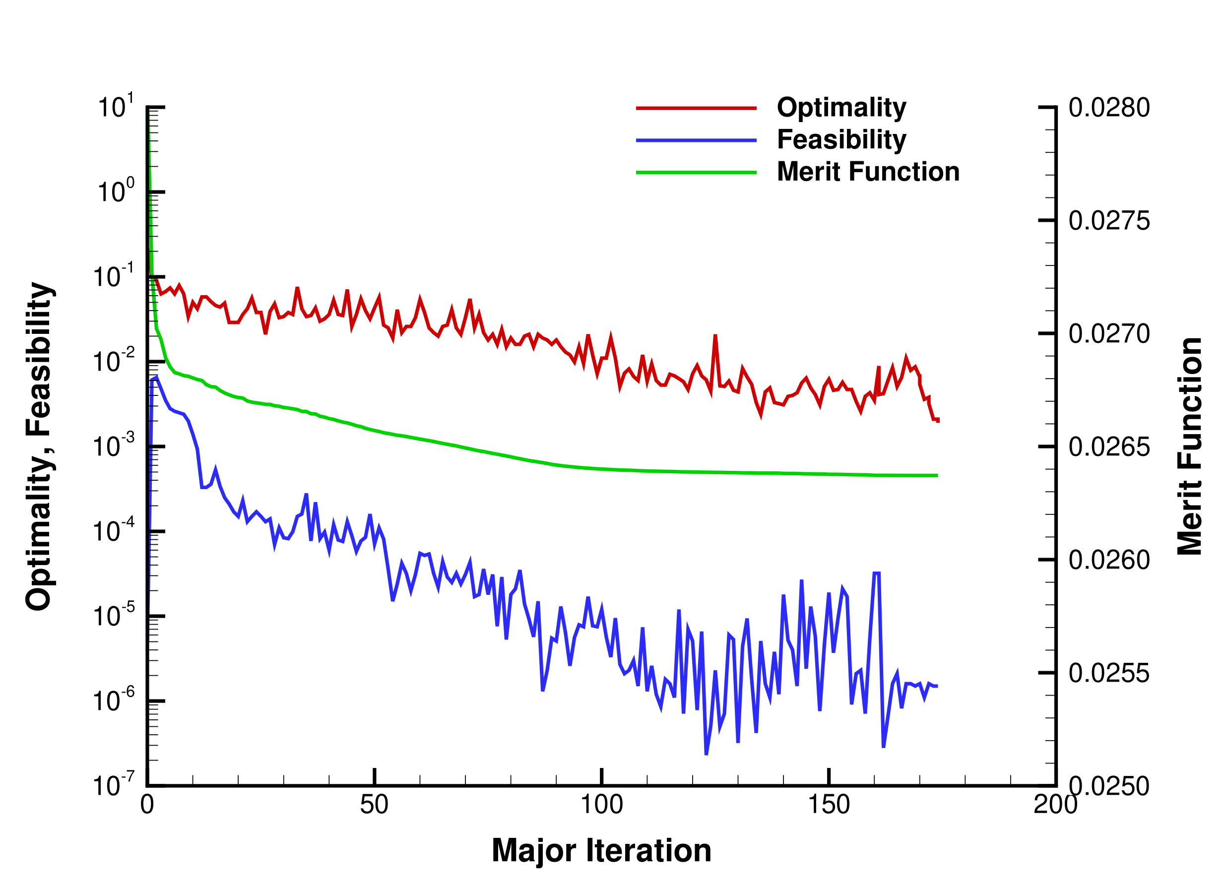
For us, this optimization problem took 56 hours on 8 Turin Athena Nodes (8 x 256 CPUs) to complete 272 function evaluations, after which SNOPT exited with
 SNOPTC EXIT  40 -- terminated after numerical difficulties
 SNOPTC INFO  41 -- current point cannot be improved
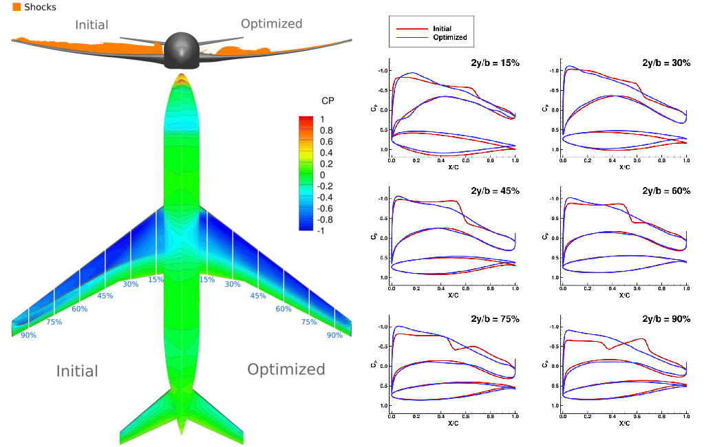
This is not uncommon for a large optimization problem such as this one. Through analysis of the optimization results, iteration number 182 was chosen as the final design. The following table and figure provide a comparison between the initial design and the chosen optimized design (iteration 182).
| Initial Value | Optimized Value | |
|---|---|---|
| Drag Coefficient \(C_D\) [counts] | \(280.6\) | \(263.7\) |
| Lift Coefficient \(C_L\) | \(0.5000\) | \(0.5000\) |
| Pitching Moment Coefficient \(C_M\) | \(-5.073 \times 10^{-6}\) | \(7.484 \times 10^{-7}\) |
| Angle of Attack | \(2.653\) | \(3.500\) |
| Tail Angle | \(-0.2848\) | \(-1.109\) |
SNOPT also provides a history of the optimization process, which is visualized in the following figure.
Relevant Publications
-
Gray, J. S., Hwang, J. T., Martins, J. R. R. A., Moore, K. T., and Naylor, B. A., "OpenMDAO: An Open-Source Framework for Multidisciplinary Design, Analysis, and Optimization," Structural and Multidisciplinary Optimization, Vol. 59, No. 4, 2019, pp. 1075--1104. https://doi.org/10.1007/s00158-019-02211-z ↩
-
Yildirim, A., Jacobson, K. E., Anibal, J. L., Stanford, B. K., Gray, J. S., Mader, C. A., Martins, J. R. R. A., and Kennedy, G. J., "MPhys: A Modular Multiphysics Library for Coupled Simulation and Adjoint Derivative Computation," Structural and Multidisciplinary Optimization, Vol. 68, No. 15, 2025. https://doi.org/10.1007/s00158-024-03900-0 ↩
-
Wu, E., Kenway, G., Mader, C. A., Jasa, J., and Martins, J. R. R. A., "[pyOptSparse:]{.nocase} A Python Framework for Large-Scale Constrained Nonlinear Optimization of Sparse Systems," Journal of Open Source Software, Vol. 5, No. 54, 2020, p. 2564. https://doi.org/10.21105/joss.02564 ↩