Block-Structured Octree Meshing
This page documents the grid { } block of the Cartesian solver inputs: the octree grid fundamentals, the two approaches to sizing the grid, user-prescribed refinement regions, and solution-based adaptive mesh refinement. For the remaining input sections see General Setup.
Basic Octree Grid Setup
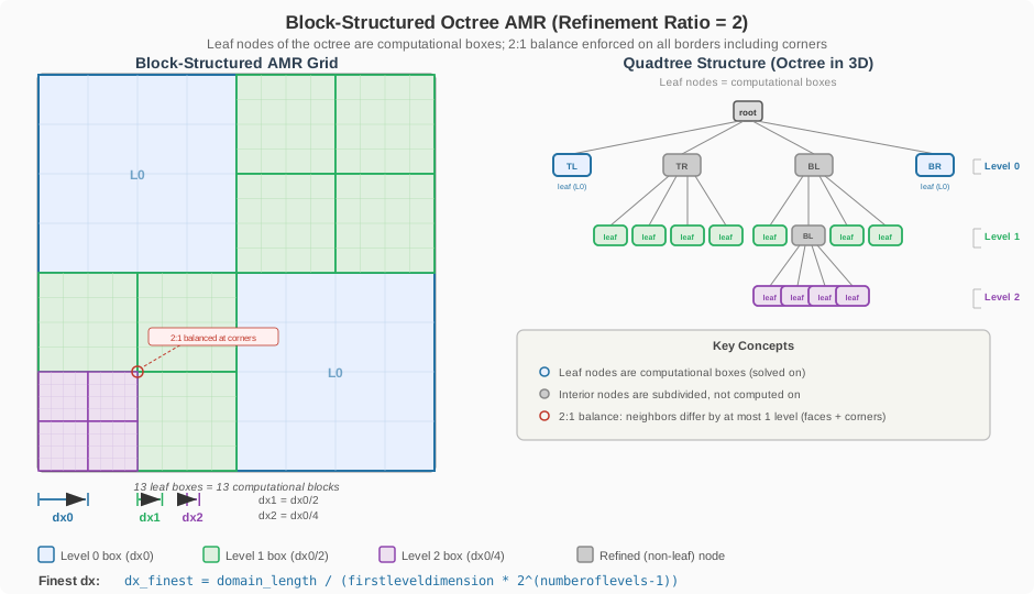
LAVA Cartesian gridding is achieved with a block-structured adaptive mesh refinement (AMR) approach using a forest of octrees. The domain is divided into a Cartesian lattice of grid points grouped into boxes, and locally refined by a factor of 2 between coarse and finer levels of refinement. Refinement can be targeted by user-prescribed regions (geometry components and volumetric tag regions) and/or driven dynamically by solution-based error metrics — both are described further down this page.
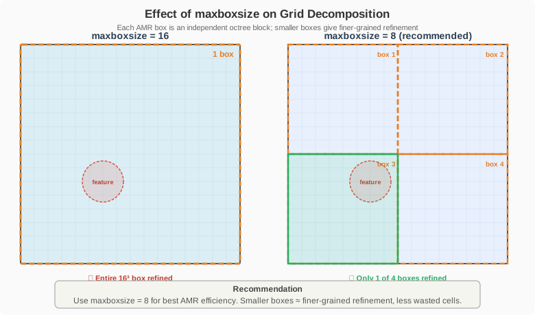
We define "boxes" as groups of cells, each containing \(N^d\) cells where \(d\) represents the spatial dimension and \(N\) is max box size. We recommend using max box size = 8, so each box contains \(8^3 = 512\) cells in 3D (or \(8^2 = 64\) cells in 2D). Mesh refinement is applied at the box level; thus, all cells within a box share the same refinement level—if any cell in a box requires refinement, the entire box is refined.
A Uniform Single-Level Grid
The simplest grid is a single-level uniform lattice:
  grid
  {
    number of levels       = 1
    max box  size          = 8
    first level dimension  = [256^3]
    domain min             = [0., 0., 0.]
    domain max             = [ 1.,  1., 1.]
  }
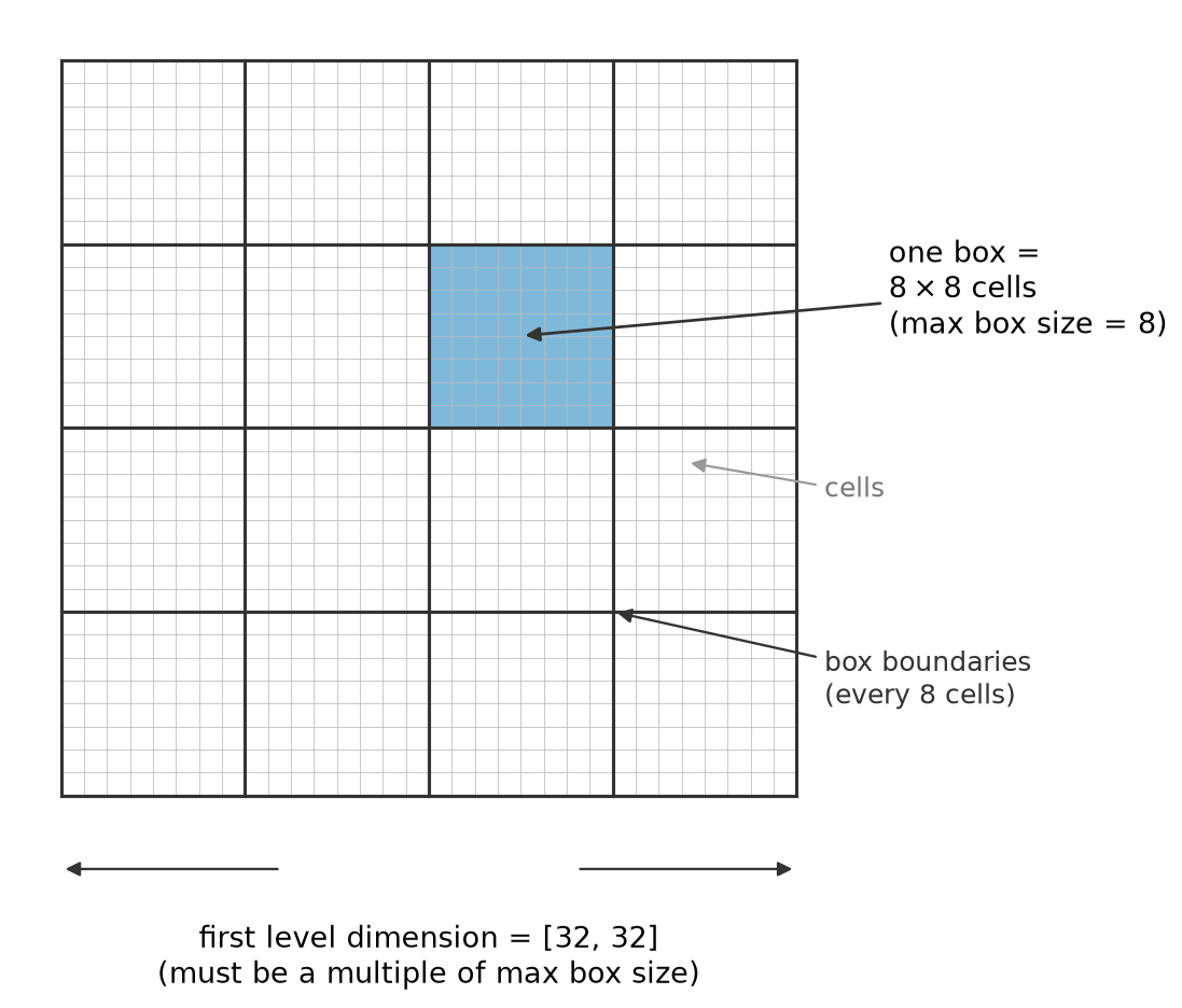
Here we define a grid of 256 cells in each spatial dimension on a 3D domain, resulting in a uniform grid with \(256^3 = 16,777,216\) cells in total. The domain extends from \([0,0,0]\) to \([1,1,1]\), and with a box size of 8, each box contains \(8^3 = 512\) cells. Since only one refinement level (number of levels = 1) is specified, the entire grid maintains a uniform refinement level throughout the domain. It's important to note that first level dimension must evenly divide by max box size. If specifying a non-cubic domain (or non-square in 2-dimensions) grids the cells must remain cubes, so \(dx = dy = dz\). We also showcase a common shorthand used in input files, where [256^3] is equivalent to explicitly writing out [256,256,256].
The sketch below shows the cell/box relationship for a smaller example (32 cells per side, boxes of 8):
Refinement Levels and Nesting
Additional levels refine the grid locally with a fixed refinement ratio of 2: each successive level halves the cell spacing relative to its parent, and fine levels nest inside coarser ones. The following diagram illustrates how refinement levels relate to each other:
Sizing the Grid: Inside-Out or Outside-In
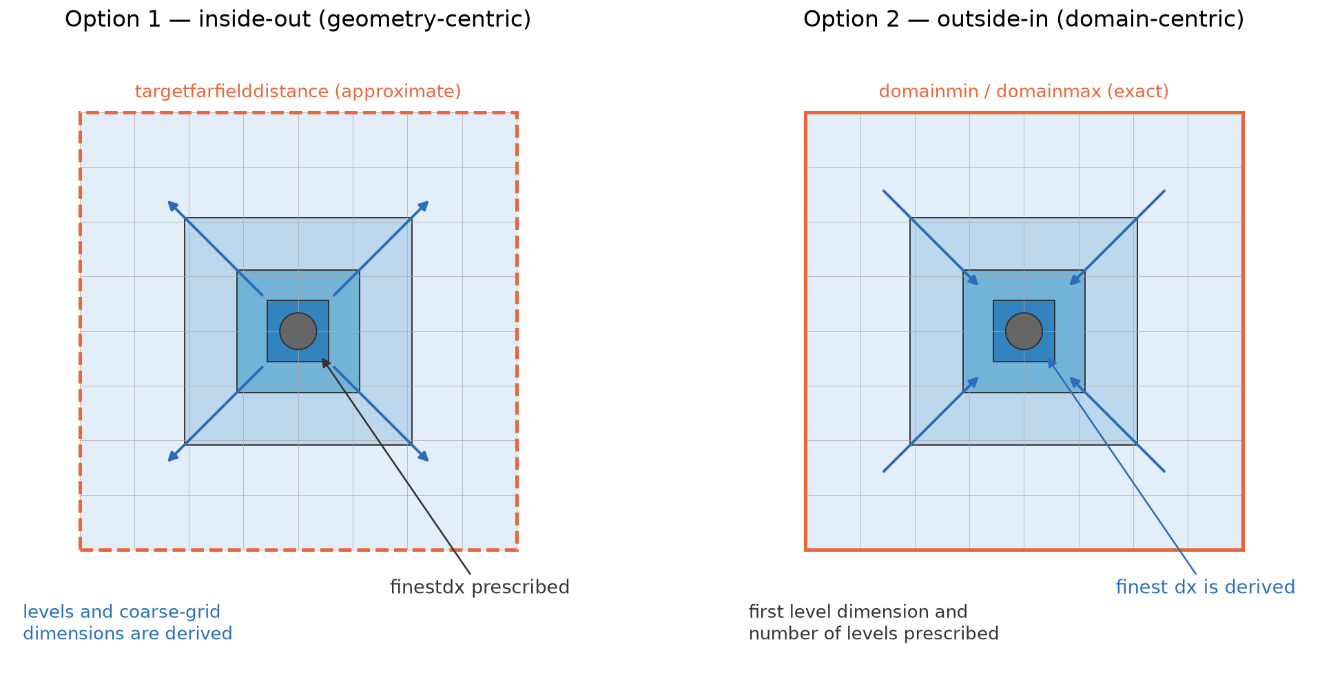
Beyond the uniform example above, every case has to answer the same question: which grid quantities do you prescribe, and which do you let the solver derive? There are two approaches:
- Option 1 — inside-out (geometry-centric). You prescribe the finest cell spacing — the quantity you actually care about near the geometry — plus a target farfield distance. The solver derives the number of levels and the coarse-grid dimensions to reach the farfield; the domain extent is rounded to fit the box and level arithmetic. The finest spacing is exact, the extent is approximate.
- Option 2 — outside-in (domain-centric). You prescribe the exact domain extents, the coarse-grid lattice, and the level budget. The finest achievable spacing is a consequence. The extent is exact, the finest spacing falls out.
Option 1: Inside-Out — Prescribe the Finest Spacing
If you specify finestdx or finestdx_rel, the solver will automatically determine the number of refinement levels and grid dimensions to achieve the requested finest cell size.
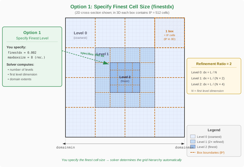
grid {
    finestdx = 0.002
    targetrelativefarfielddistance = [100, 100, 100] # Optional: farfield distance relative to reference length
    targetfarfielddistance = [100, 100, 100]         # Optional: absolute farfield distance
    domainorigin = [0.0, 0.0, 0.0]                   # Optional: shifts the assembled domain
    aligndomainfacetoorigin = [none, lo, none]       # Optional: anchor a domain face at the origin (halves the domain)
    maxboxsize = 8
}
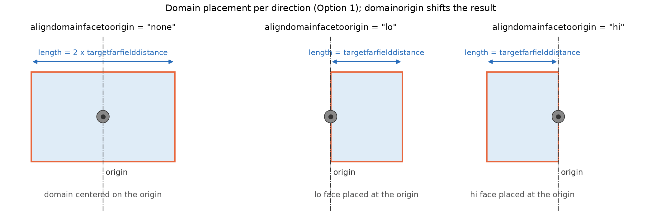
finestdx: Target finest cell size (required for minimal input).finestdx_rel: Replacesfinestdxif present. Target finest cell size factor relative to the referencedx(defined in the reference section).targetrelativefarfielddistance: Farfield distance relative to reference length (overridestargetfarfielddistanceif present).targetfarfielddistance: Absolute farfield distance.aligndomainfacetoorigin: Per directionnone,lo, orhi. Withnonethe domain is centered on the origin and its total length in that direction is \(2\times\) the farfield distance. Withlo(hi) the low (high) domain face is placed exactly at the origin and the domain extends only to one side, with length equal to the farfield distance — the domain is halved, which is the natural setup for symmetry planes and ground planes.domainorigin: Shifts the assembled domain by this point, i.e. the domain center (or the aligned face) ends up atdomainorigininstead of the coordinate origin.
Note
The placement keys (targetfarfielddistance, domainorigin, aligndomainfacetoorigin) belong to the inside-out approach only, where the solver assembles the domain around the geometry. In the outside-in approach the domain placement is given directly and exactly by domainmin / domainmax.
Option 2: Outside-In — Prescribe the Domain and Level Budget
Alternatively, you can specify the grid dimensions and number of levels directly:
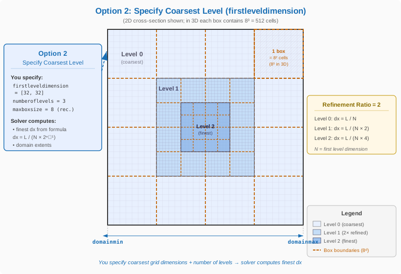
grid {
    firstleveldimension = [128, 128, 128]  # Number of cells in each direction on the coarsest grid
    numberoflevels = 3
    domainmin = [0.0, 0.0, 0.0]
    domainmax = [1.0, 1.0, 1.0]
    maxboxsize = 8
}
firstleveldimension: Number of cells in each direction on the coarsest grid (must be a multiple ofmaxboxsize).numberoflevels: Number of AMR levels.domainmin,domainmax: Physical extents of the domain.
The finest spacing follows from the level budget:
Common Grid Keys and Constraints
The following keys apply to either sizing approach:
maxboxsize: Number of cells per box per direction. Recommended value: 8 (i.e., \(8^3 = 512\) cells/box in 3D). Must be at least 4 if using refinement.grid_scale: Global scale factor (default: 1.0) applied to every geometric length in thegridsection:finestdx, the farfield targets, the domain extents and origin, and all tag-region coordinates, radii, and spacings. Useful when the geometry is modeled in different units than the flow problem. It multiplies the final values — i.e. after any*_relscaling by the referencedx— and does not modify the referencedxitself.
Constraints to keep in mind:
- All grid dimensions must be integer multiples of
maxboxsize. - For periodic boundary conditions, at least 2 boxes per direction are required.
- The refinement ratio between levels is fixed at 2.
- Cells must be isotropic (\(dx = dy = dz\)); if the aspect ratio is not unity and
nonunitokis not set, the code will stop with an error.
The Three Spacing Inputs
Spacing appears in three different places of the input file, and mixing up their roles is the most common source of confusion in the Cartesian grid setup:
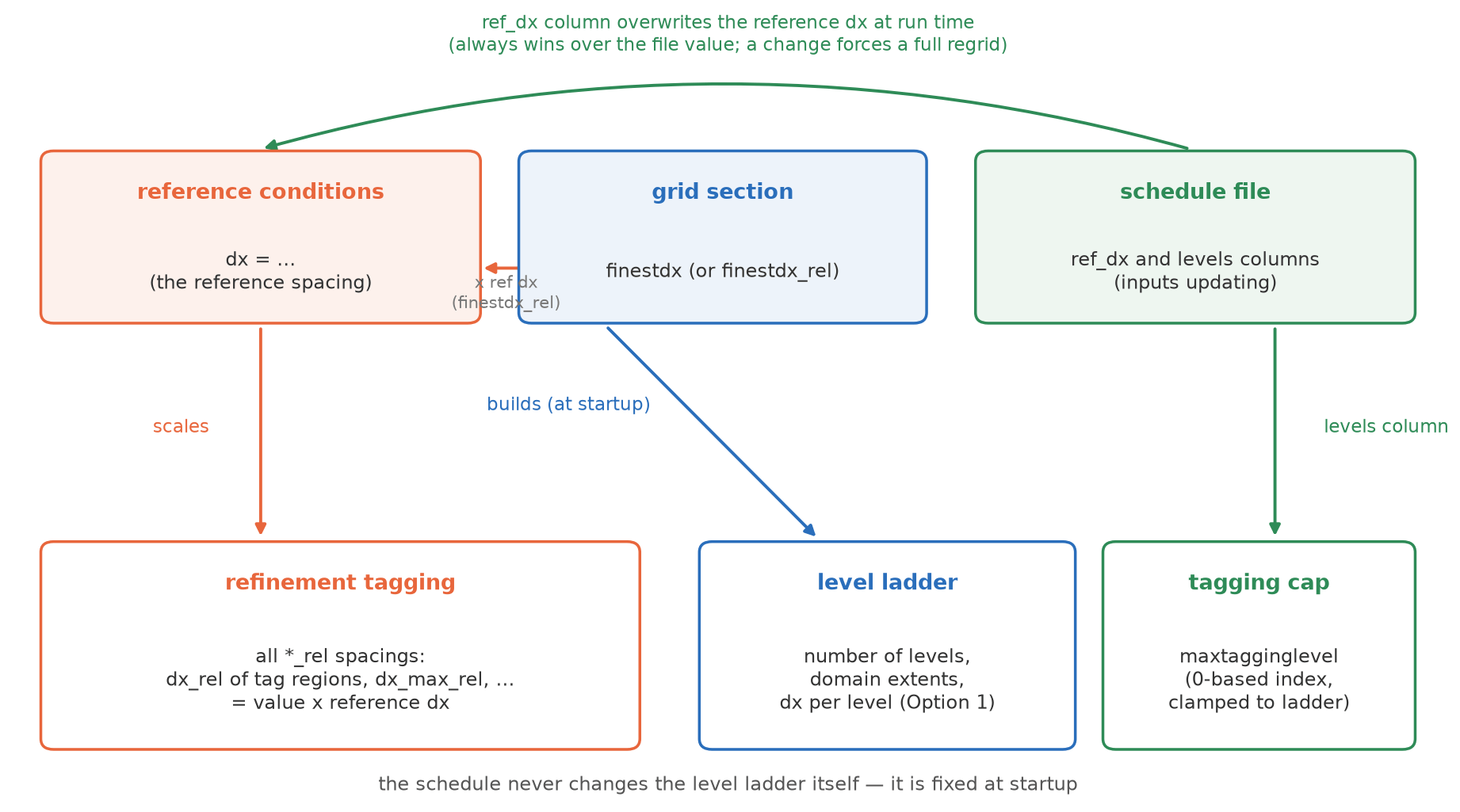
dxin thereference conditionssection — the reference spacing. A pure scale factor: every*_relspacing key (dx_relof tag regions,finestdx_rel,dx_max_relof a telescoping frustum, ...) is multiplied by it. Absolute keys (dx,finestdx,dx_max) ignore it entirely.finestdxin thegridsection — the ladder builder. Used only at startup, in the inside-out approach, to construct the level ladder: the number of levels, the domain extents, and the per-level spacings. It takes no part in any tagging decision — tagging compares each cell's level spacing against the tag's requesteddxand refines until the request is met or the ladder (or the tagging cap) ends. Its only connection to tagging is that it defines what "finest" means fordx = 0.0tags.- The schedule file (
inputs updating) — runtime control. Two schedule columns interact with the spacings:- The
ref_dxcolumn (do ref dx = true) overwrites the referencedxwhile the run advances. On every update interval the input file is completely re-read and all*_relspacings are re-derived from the scheduled value. Once the scheduler has set the referencedx, thedxin thereference conditionssection is ignored for the rest of the run. A change in the scheduled value forces a full regrid at the next opportunity, independent ofregridinterval. - The
levelscolumn (do levels = true) moves the maximum tagging level (maxtagginglevel, a 0-based level index) — it does not add or remove actual levels. The level ladder is fixed at startup; a request beyond the ladder is clamped with a warning. Like a scheduledref_dxchange, a change of the cap (or of a scheduledmaxcellsbudget) forces a full regrid at the next step rather than waiting forregridintervalto elapse — regridding must still be enabled (regrid interval> 0).
- The
The two combinations that come up most often:
- Absolute-
dxtags with a levels-only schedule ("add a level every N CTUs"): the tags keep the spacing they request throughout — raising thelevelscolumn simply lets them reach the finer ladder levels that were capped before, with the regrid happening right at the scheduled step. The referencedxnever changes. dx_reltags with aref_dxschedule (grid sequencing): halving the scheduled referencedxhalves everydx_rel-based tag spacing at the next update interval and triggers the regrid. This is the mechanism behind single-run grid refinement studies (see the schedule file documentation and the CRM-HL tutorial).
Warning
The level ladder is built before the first schedule row is applied, from the grid section and the file's reference dx. When scheduling ref_dx down toward a fine target, make sure the startup ladder is already deep enough for the finest scheduled spacing (e.g. size finestdx or number of levels for the final target) — tags finer than the ladder's finest level are silently clamped to it.
User-Prescribed Refinement Regions
Refinement can be targeted to specific regions of the domain by tagging. The diagram below illustrates the main tagging methods:

A few conventions shared by all tag regions:
- Each region requests a target spacing with
dx, or withdx_relas a factor relative to the referencedx(defined in the reference section). Settingdx = 0.0requests the finest resolution available, defined either byfinestdxor the maximum number of refinement levels. - Regions are enumerated per type —
tagboxes_1,tagboxes_2,tagcylinders_1, … — and any combination of types and counts may be used together. - Every region accepts an optional activation window
nton/ntoff: the region only tags whilenton\(\le\)nt\(\le\)ntoff(time step count), which is useful for startup refinement that should later be released. - For inspection, the prescribed tag points, boxes, cylinders, and spheroids are dumped as VTK files into the
tags/directory of the run.
Component Tagging
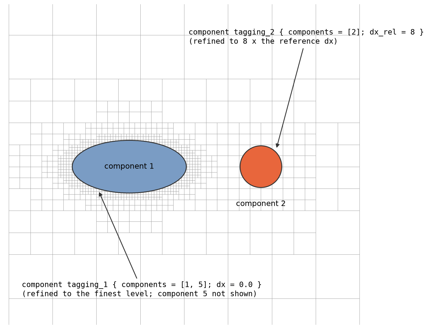
Refinement regions can be tied to the input geometry using the component numerical values of the surface triangulation (see the Geometry section). For example:
component tagging_1 { components = [1, 5]; dx = 0.0 }
component tagging_2 { components = [2]; dx_rel = 8 }
The first section refines the cells adjacent to the surfaces of components 1 and 5 to the finest available resolution; the second refines the cells around component 2 to \(8\times\) the reference dx. Optionally, type = edge restricts the tagging to the components' feature edges instead of the full surfaces (type = component is the default).
Tag Boxes
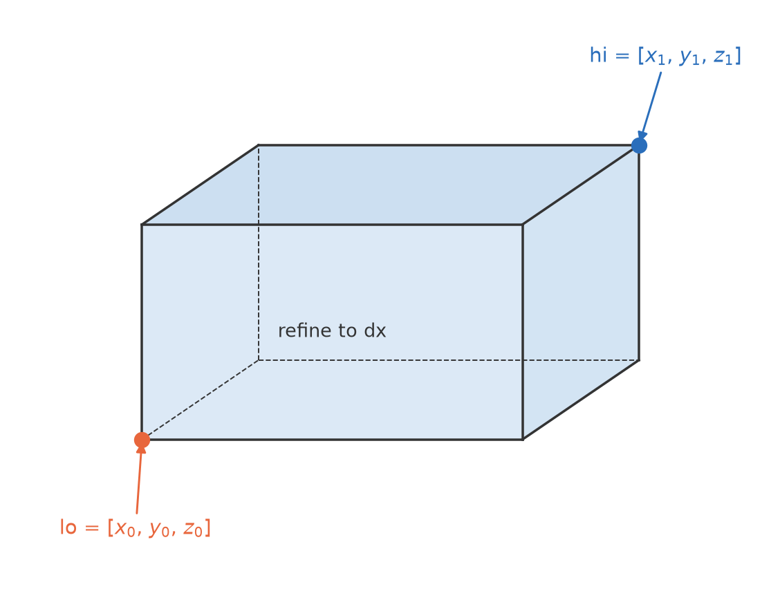
Refinement can be targeted within explicitly defined rectangular regions (tagboxes):
This specifies a rectangular region from lo to hi coordinates, refined to a grid spacing (dx) of 0.4 (dx_rel works as well).
Tag Cylinders
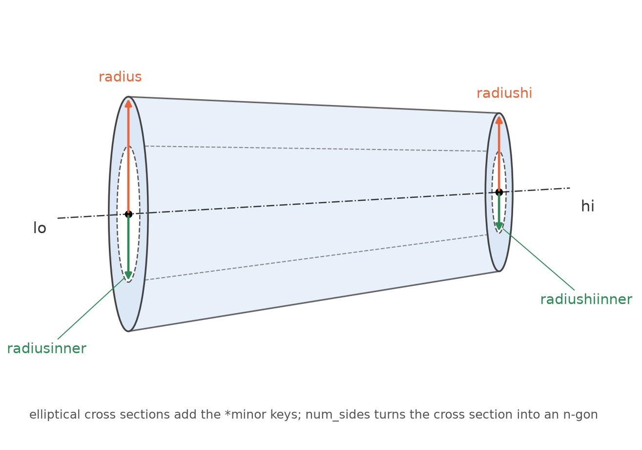
Cylindrical refinement regions can be defined using the tagcylinders parameter. Each cylindrical region is specified with the following parameters:
tagcylinders_1 { lo = [0, 0, 0]; hi = [3, 0, 0]; radius = 2.24517; radius hi = 3.367785; dx = 0.0325 }
dx(ordx_rel): Target spacing inside the region;dx_relis multiplied by the referencedx.lo: Coordinates of the cylinder's bottom center point.hi: Coordinates of the cylinder's top center point.radius: Radius at the cylinder's bottom (lopoint).radiusinner: Inner radius at the cylinder's bottom, defining a hollow cylindrical region. Defaults to0.0if not specified.radiushi: Radius at the cylinder's top (hipoint). Defaults to the bottom radius (radius) if not specified.radiushiinner: Inner radius at the cylinder's top, defining the upper inner radius of a hollow cylindrical region. Defaults to the bottom inner radius (radiusinner) if not specified.
Note
Make an inner cutout comfortably larger than the AMR boxes of the refinement levels it must survive on: refinement acts on whole boxes and tags are grown by regridgrowtags cells, so a hole only one or two boxes wide fills in and can appear as if the inner radius were ignored. For n-gon cross sections the radii are circumradii, i.e. the flat-to-flat half-width of the cutout is only \(r\cos(\pi/n)\).
Since radius and radiushi may differ, a tag cylinder is in general a conical frustum. The cross section does not have to be circular:
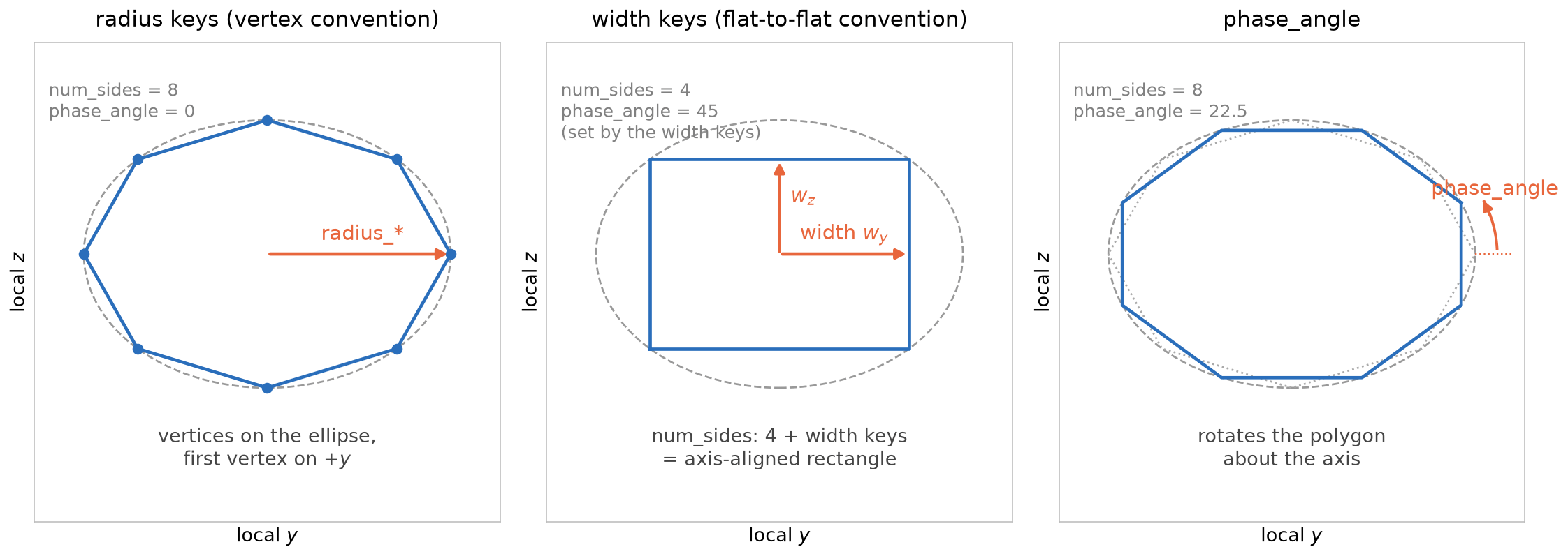
radiusminor,radiushiminor,radiusinnerminor,radiushiinnerminor: Minor-axis radii of an elliptical cross section, one per radius above. Each defaults to its corresponding (major) radius, which recovers the circular cross section. The major radii span the first transverse direction of the axis frame and the minor radii the second; the frame convention matches the LAVA Voronoi mesher'sfrustumregion, so identical inputs produce identical shapes in both meshers.num_sides:0(default) keeps the circular/elliptical cross section; a value>= 3replaces it with a regular n-gon whose circumradius is given by the radii above (stretched by the major/minor aspect ratio).phase_angle: Rotation of the n-gon about the axis in degrees. With the default of0the first vertex sits on the major axis — sonum_sides = 4gives a square standing on its corner (a rhombus). To align the flats with the axes — e.g. an axis-aligned rectangular duct — setphase_angle = 45fornum_sides = 4(in general \(180/\)num_sides). Requiresnum_sides >= 3.
For example, an axis-aligned rectangular duct: a square cross section stretched to a 3:2 major/minor aspect ratio, with phase_angle = 45 placing the flats on the axes — the shape shown in the telescoping-frustum figures below:
tagcylinders_2 {
  dx          = 0.02
  lo          = [0.0, 0.0, 0.0]
  hi          = [3.0, 0.0, 0.0]
  radius      = 0.6;  radiushi      = 0.9   # major radii at the lo and hi caps
  radiusminor = 0.4;  radiushiminor = 0.6   # minor radii: elliptical 3:2 aspect
  num_sides   = 4                           # square cross section...
  phase_angle = 45.0                        # ...with its flats aligned to the axes
}
The radius and phase conventions are identical to the Voronoi mesher's frustum region:
Note
The flat-to-flat width keys shown in the middle panel are currently a Voronoi-mesher-only input; the Cartesian tag cylinders use the radius (circumradius) keys.
Elliptical and n-gon cross sections require a 3D build.
Tag Spheroids
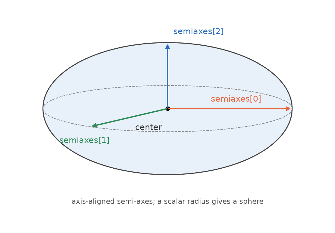
Ellipsoidal refinement regions are defined with tagspheroids, using axis-aligned semi-axes (or a scalar radius for a sphere):
dx(ordx_rel): Target spacing inside the region;dx_relis multiplied by the referencedx.center: Center point of the spheroid.semiaxes: Semi-axes along the coordinate directions; all equal recovers a sphere.radius: Scalar alternative tosemiaxesfor a sphere.
Telescoping Frustum
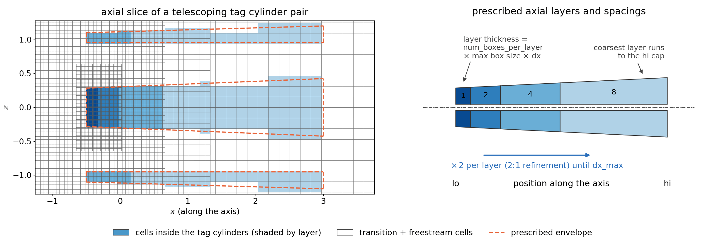
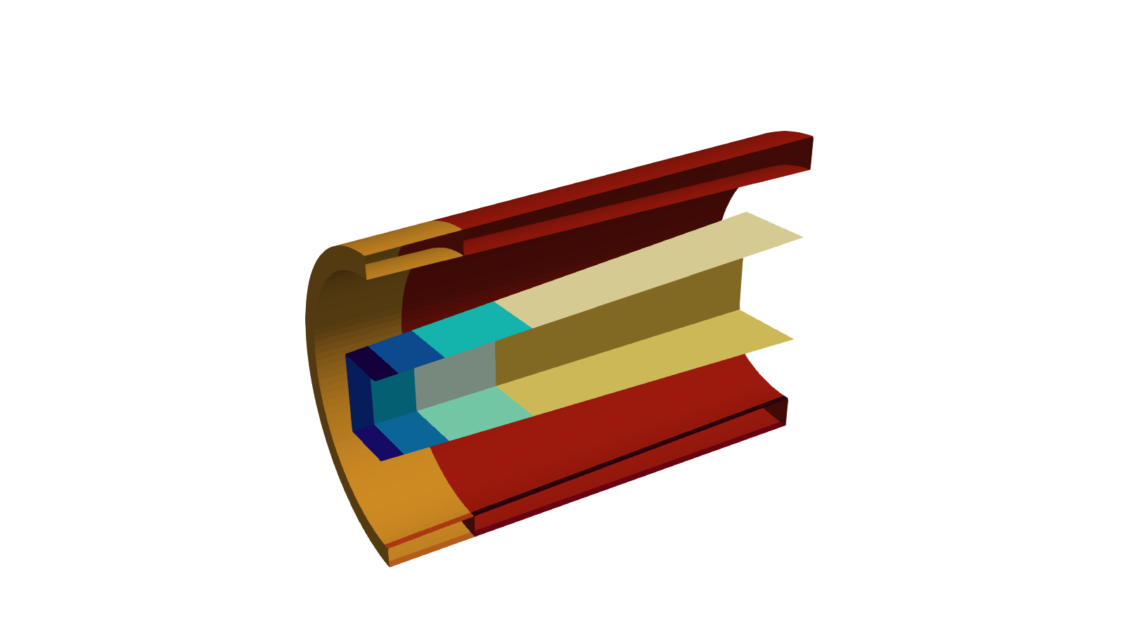
For jet-type simulations the cell size should grow gradually along the plume to avoid abrupt cell-volume changes near the shear layer while keeping the cell count affordable. Instead of hand-stacking tag cylinders, a telescope_axial sub-section turns a single tag cylinder definition into a telescoping frustum: refinement layers march from the lo cap along the axis, and every layer doubles the grid spacing (matching the 2:1 refinement ratio of the Cartesian octree) until the requested maximum spacing is reached. The layer thickness is specified in AMR blocks of the layer's own spacing, so layers align naturally with the block structure. The coarsest layer extends to the hi cap. The finest layer always starts at the lo cap, and there is no ordering requirement between the two points — swapping lo and hi reverses the telescoping direction, and the axis may point in any direction. The outer, inner, major, and minor radii of each layer are interpolated linearly along the enclosing frustum definition, so annular (hollow) and n-gon telescopes work the same way as plain tag cylinders. This is the Cartesian counterpart of the Voronoi mesher's telescoping_frustum region; the octree's automatic 2:1 grading replaces that region's explicit radial_refinement rings.
tagcylinders_1 {
  dx     = 0.04                     # spacing of the first (finest) layer at the lo cap
  lo     = [-0.5, 0.0, 0.0]
  hi     = [ 3.0, 0.0, 0.0]
  radius = 0.6; radiushi = 0.9      # frustum envelope; inner/minor radii and num_sides work as usual
  telescope_axial {
    dx_max              = 0.16      # coarsest spacing; dx_max_rel is also supported
    num_boxes_per_layer = 2         # layer thickness = 2 AMR blocks of the layer's dx
  }
}
dx_max(ordx_max_rel): Spacing of the coarsest layer; layer spacing doubles from the tag cylinder'sdxuntil this value.num_boxes_per_layer: Thickness of each layer in AMR blocks (max box sizecells) of that layer's spacing.num_boxes_per_layer_growth(default1): Factor applied to the box count of each subsequent layer, rounded to the nearest integer and never below one block. Since the spacing doubles per layer, the default of1doubles the physical layer thickness each time;0.5keeps the physical thickness (approximately) constant along the axis;2quadruples it.stretch_ratio: Alternative tonum_boxes_per_layer(specify exactly one). Emulates a smooth geometric stretching with the given ratio, as familiar from curvilinear meshing: the number of cells over which such a stretching doubles the spacing, \(\ln 2/\ln r\), is converted to the equivalent whole number of blocks per layer. For example,stretch_ratio = 1.05gives \(14.2\) cells \(\approx 2\) blocks of 8. Because of the rounding the achieved effective ratio differs from the request (it is reported in the log); very aggressive ratios saturate at one block per layer.
Outward Telescoping
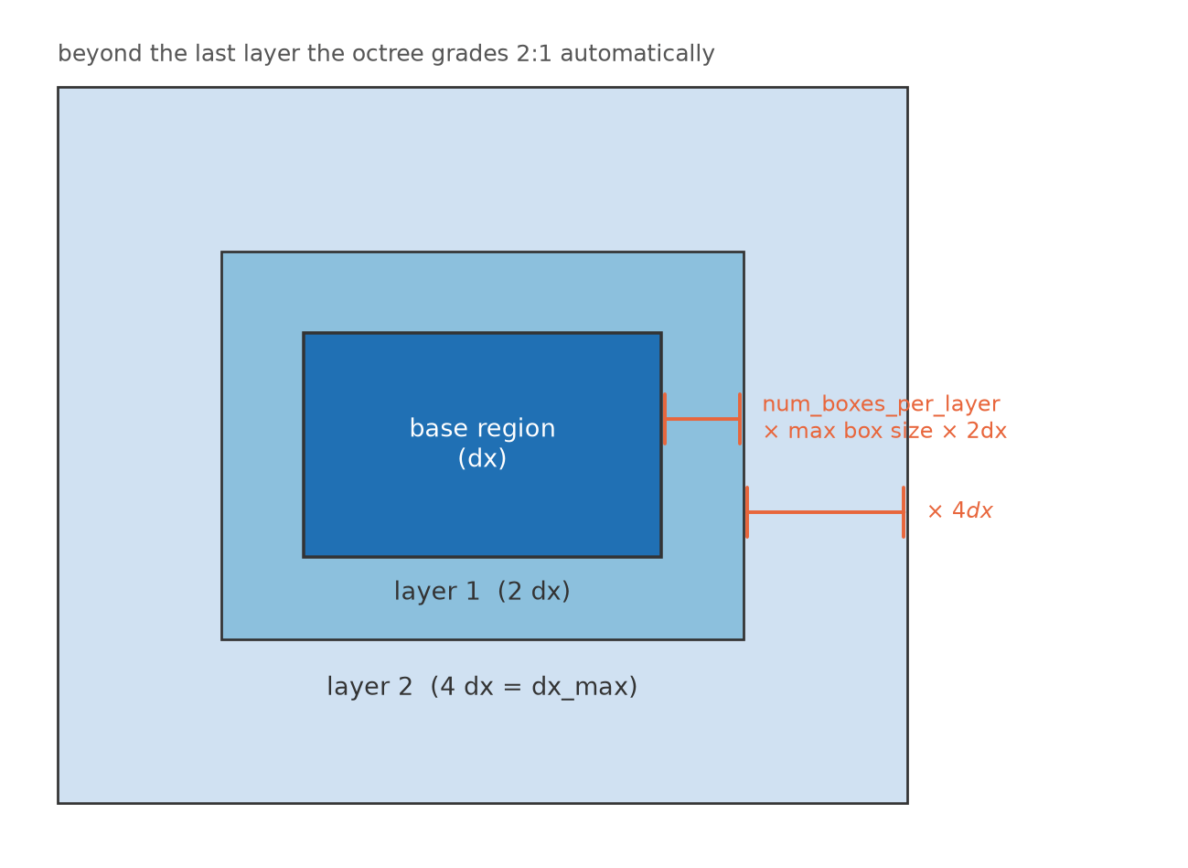
Any tag box, cylinder, or spheroid can carry a telescope_outward {} sub-section. The base region keeps its spacing, and dilated copies of the shape wrap it on all sides with the spacing doubling per layer until dx_max is reached — after the last layer the octree's automatic 2:1 grading takes over toward the freestream. A box grows by the layer offset at all corners; a cylinder grows its radii and extends its axis (an annular cutout shrinks and eventually closes); a spheroid grows its semi-axes. This is the Cartesian counterpart of the Voronoi mesher's telescoping_refinement section, and it controls how much volume every intermediate refinement level occupies instead of leaving only the minimal nesting buffer.
tagboxes_1 {
  lo = [-1, -1, -1]; hi = [1, 1, 1]; dx = 0.02
  telescope_outward {
    dx_max              = 0.16   # coarsest layer spacing; dx_max_rel also supported
    num_boxes_per_layer = 2      # or stretch_ratio; num_boxes_per_layer_growth optional
  }
}
The layering keys (dx_max/dx_max_rel, num_boxes_per_layer, stretch_ratio, num_boxes_per_layer_growth) work exactly as for the telescoping frustum. The telescoping is resolved once at input time into ordinary tag regions, so regridding sees no additional machinery — the generated layers are visible in the tags/ VTK dumps.
Tag Points
Pointwise tagging can also be utilized (remember, the entire box will be subject to the smallest tagged cell).
Adaptive Mesh Refinement Setup
The Cartesian solver supports solution-based AMR tagging using a variety of error metrics and field-based thresholds. These options allow you to refine the mesh dynamically in regions where the solution exhibits sharp gradients or other features of interest.
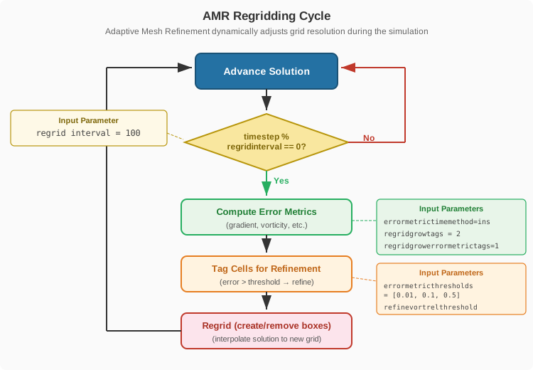
Regridding Cadence
The following grid-section keys control how often the grid adapts:
regridinterval: Number of steps between regridding operations; larger is better for performance.regridintervalon,regridintervaloff: Control regridding intervals for on/off cycles.regridgrowtags: Grows the refined region around geometry tags by the given number of cells.regridgrowerrormetrictags: Grows the refined region around error-metric tags by the given number of cells.
Quick-Start Examples
Solution-based AMR with user-specified thresholds:
    grid {
        finest dx = 0.008 # finest level based approach
        targetrelativefarfielddistance = [200,100^2]  # distance from origin to farfield BC in units of reference length
        aligndomainfacetoorigin = [none, none, none]
        max box size = 8
        regrid interval = 100 # number of time steps between regrids, larger is better for performance
        regridgrowtags = 2 # increases amount of refined boxes around geometry by 2 cells

        solution based amr
        {
          method = user
          errormetric_1 {type=smallscaleenergy; weight=1.0}
          errormetricgeomdistancescalingreflength = 22.5
          errormetricthresholds = [0.0000125, 0.000025, 0.00005, 0.000125, 0.00025, 0.0005, 0.00100, 0.0025, 0.005, 0.01, 0.04, 0.12, 0.24, 0.48, 0.96]
          regridgrowerrormetrictags = 1
        }
    }
The same setup with automatically determined thresholds:
    grid {
        finest dx = 0.008 # finest level based approach
        targetrelativefarfielddistance = [200,100^2]  # distance from origin to farfield BC in units of reference length
        aligndomainfacetoorigin = [none, none, none]
        max box size = 8
        regrid interval = 100 # number of time steps between regrids, larger is better for performance
        regridgrowtags = 2 # increases amount of refined boxes around geometry by 2 cells

        solution based amr
        {
          method = auto
          errormetric_1 {type=smallscaleenergy; weight=1.0}
          errormetricgeomdistancescalingreflength = 22.5
          regridgrowerrormetrictags = 1
        }
    }
Specifying Error Metrics
The specification of error metrics is achieved through enumerated subsections errormetric_* {} within the solution based amr {} subsection. For example, two error metrics may be specified as follows:
grid
{
  solution based amr
  {
    errormetric_1 {type = laplacianp; weight = 0.5}
    errormetric_2 {type = laplaciant; weight = 0.5}
  }
}
Options include:
typeError metric name. Default:smallscaleenergy.weightWeight to apply to the specified error metric across all levels. Default: 1.0weightsperlevelArray of length equal to the number of AMR levels, specifying the weight to use on each level. If bothweightandweightsperlevelare provided, thenweightsperlevelwill be used. Default: [1.0,1.0,...,1.0]
Types of error metrics:
-
laplacianpRefine based on the Laplacian of pressure. -
laplacianu,laplacianv,laplacianwRefine based on the Laplacian of velocity components (u, v, w). -
laplaciant(single phase only) Refine based on the Laplacian of temperature. -
smallscaleenergyRefine based on small-scale energy content. -
leonardstressmagRefine based on the Leonard stress magnitude. -
chuenergynormRefine based on the Chu energy norm. -
vortrelRefine based on relative vorticity magnitude. -
tkeRefine based on turbulent kinetic energy (TKE). -
prmsRefine based on pressure RMS. -
heatreleaserate(reacting flows only) Refine based on the heat release rate. -
maxmixing(multispecies only) Refine based on maximum mixing fraction.
Thresholds, Budgets, and Metric Accumulation
The solution based amr {} subsection accepts the following options:
methodAMR thresholding method. Options include:user: Users must provide thresholds viaerrormetricthresholdfinestorerrormetricthresholds.auto: Refinement and coarsening thresholds are automatically determined using distribution thresholding.-
none: Solution-based AMR is turned off. -
errormetricthresholdfinestSet fixed error metric threshold per level based on the value for which the mesh should be refined to the finest available. The thresholds for coarsening and refinement for each level will then be automatically populated using the ratio to obtain the next coarsest refinement levelerrormetricthresholdratiowhich defaults to 0.5 to reduce mesh size as much as possible with minimal impact to solution accuracy -
errormetricthresholdminMin allowed threshold for solution based amr tagging. This is to avoid chasing non-physical error metrics. Default is 0.001. -
errormetricthresholdsSet fixed error metric thresholds per level (overrides the above if present). -
thresholddomainextentSpecifies whether to use the maximum or mean error as the maximum possible threshold value. Options:maxerror(use max error as the upper bound of threshold domain, default)meanerror(use mean error as the upper bound of the threshold domain)
-
maxcellsMaximum total number of cells. This limit is enforced when either user-specified thresholds or automated distribution thresholds are estimated to result in a total cell count exceeding the number specified. Example:maxcells = 150000000. -
maxcellstoleranceThe convergence criteria for the max cells constraint. For example, if 0.01 is specified, then we terminate the search when we have a set of thresholds that are 1% below the specified cell limit. Default:0.015. -
maxitercelllimitsearchThe maximum number of iterations to perform when searching for error thresholds that satisfy the imposedmaxcellsconstraint. Default:50. -
maxmemorypercenthostThe maximum percentage of host memory to utilize. This parameter is used at each adaptation cycle to generate an approximate limit on the number of cells we can afford to increase our grid size by. Default:80. -
maxmemorypercentgpuThe maximum percentage of GPU memory to utilize. This parameter is used at each adaptation cycle to generate an approximate limit on the number of cells we can afford to increase our grid size by. Default:80. -
enforcemaxmemorylimitAdjusts the user-specifiedmaxcellsparameter if memory usage will exceedmaxmemorypercenthostandmaxmemorypercentgpu. Warning this capability is currently under development and may result in undesired behavior. Default:false. -
errormetrictimemethodControls how error metrics are accumulated in time. Options:ins(instantaneous, default)avg(time average)max(maximum over time)
-
errormetricexponentialmovingaveragewindow,errormetricexponentialmovingaveragewindowctuWindow length for the exponential moving average (used iferrormetrictimemethod = avg). Thectuvariant is in convective time units; without the suffix the value is in physical time (seconds). The equivalent...timescale/...timescalectukeys are also accepted. -
errormetricresetonregridIf true, resets error metrics on each regrid. -
errormetricradialscalepoint,errormetricradialscalepowEnable and control radial scaling of error metrics. -
errormetricgeomdistancescalingreflengthReference length (\(d_0\)) for geometric distance scaling in error metrics, in meters. Scales down the error metric computed by \(1/2^{d/d_0}\) to avoid refining wakes and bow shocks all the way to the edge of the computational domain where they likely no longer affect quantities of interest. -
errormetricdogpuIf true, compute error metrics on GPU (requires at least one threshold to be set). -
errormetricstatsintervalInterval (in steps) to update error metric statistics
Notes:
- If the solution based amr section is NOT present, then no solution-based AMR is performed.
- If solution based amr is present, then the default for method is auto.
Regional Error-Metric Scaling
The error metric can be scaled inside user-defined regions, e.g. to suppress solution-based refinement in areas that are known to be uninteresting (sponge zones, far wakes), or to weight it up in areas of interest. Inside a region the metric is multiplied by its errormetricscale factor (default 0.0, i.e. solution-based refinement is fully suppressed there); the regions also accept the nton / ntoff activation window.
Boxes are defined directly in the grid section, and cylinders inside the solution based amr subsection with the full tag cylinder shape syntax:
grid
{
  errormetricscaleboxes_1 { lo = [10, -5, -5]; hi = [40, 5, 5]; errormetricscale = 0.0 }

  solution based amr
  {
    errormetricscalecylinders_1 { lo = [0,0,0]; hi = [8,0,0]; radius = 2.0; errormetricscale = 0.25 }
  }
}
Wall-Resolution Based Refinement
Refinement can also be driven by the resolved wall spacing of geometry components. The thresholds are specified as arrays of length equal to the number of AMR levels (except the base level):
refineypluscomps = [ 1-9, 10]components to use for y-plus based refinementrefineyplusthreshold = [1000^9,200]yplus threshold levels for the components
Additional Options
dumpinitgridsonly: If true, only writes initial grid and exits — useful for iterating on the grid setup without running the solver.maxtagginglevel: Maximum AMR level for tagging/refinement (default: highest level).minlevel: Minimum AMR level (default: 0).prunecoveredboxes: If true, removes boxes fully covered by finer grids.