Quick Start
This guide takes you through your first LAVA Cartesian simulation in a few minutes: the Taylor–Green vortex, a canonical transition-to-turbulence case in a periodic box. It needs no geometry, no mesh refinement, and a single small input file — the initial condition is built into the solver.
Prerequisites
Before starting, ensure you have:
- The LAVA solver and utilities installed and your environment properly set up, see the LAVA Installation Guide. You need a 3D Cartesian executable (any
3D NS1build). - Python with matplotlib for the
plotHist.pyutility.
The Case
The Taylor–Green vortex starts from a smooth, analytic vortical velocity field in a triply periodic box. The large initial vortices stretch, break down into ever smaller scales, and finally decay — making it the standard test of how much numerical dissipation a scheme adds to an under-resolved turbulent flow. In a box \(\mathbf{x} \in [0,1]^3\) with \(f = 2\pi\), the built-in initial condition is
with the corresponding pressure field
We run the classic configuration of Carton de Wiart et al. (2014): Reynolds number 1600, Mach number 0.1, on a uniform \(64^3\) grid — a deliberately coarse resolution where the quality of the numerical scheme is visible.
Reference: Carton de Wiart, C., Hillewaert, K., Duponcheel, M., & Winckelmans, G. (2014), "Assessment of a discontinuous Galerkin method for the simulation of vortical flows at high Reynolds number," International Journal for Numerical Methods in Fluids, 74(7), 469–493.
Note
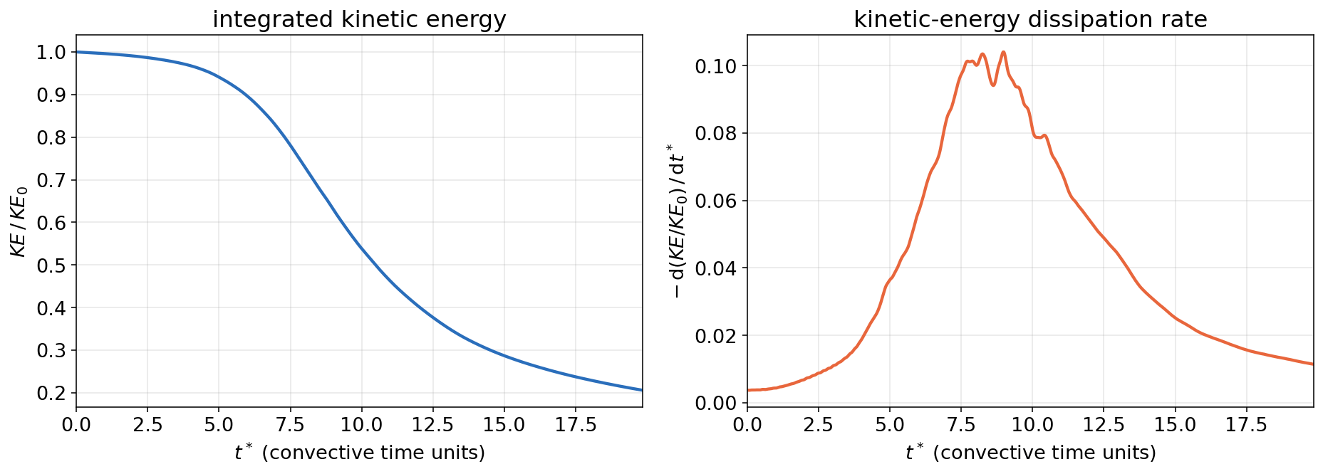
This quick start is about getting a first simulation running, not about producing a reference-quality solution: the \(64^3\) grid deliberately under-resolves the flow. Expect the results to be qualitatively right and quantitatively close — in this run the dissipation peak lands at \(t^* = 9.0\) as in the reference DNS, with its magnitude a few percent high, which is the expected coarse-grid behavior. Grid and scheme refinement studies are what the rest of the documentation is for.
Tutorial Files
Download the two input files into a working directory:
| File | Description |
|---|---|
| tgv.inputs | solver input file |
| tg.spec | gas/species definition (sets the viscosity, i.e. the Reynolds number) |
The Input File
The complete input file:
# LAVA Cartesian quick start: the Taylor-Green vortex.
# A periodic box with no geometry; the initial condition is built into the solver.
exact flow name = taylorgreenvortex

time {
  steady          = false
  number of steps = 7900   # roughly 20 convective time units at CFL 0.8
  cfl             = 0.8
}

solver defaults {
  explicit { method = ssprk33 }   # 3rd-order strong-stability-preserving Runge-Kutta
}

reference conditions {
  velocity    = [1.0, 0, 0]
  density     = 6.283185307179586    # 2 pi
  temperature = 71.4285714285714     # gives Mach 0.1
  length      = 0.15915494309189535  # 1 / (2 pi): one classic TGV time unit per ctu
}

fluid {
  species = tg   # calorically perfect gas with constant viscosity 1/1600 (Re = 1600)
}

cartesian {

  convective terms {
    scheme            = hwcns      # low-dissipation central scheme
    fluxfunction      = ausmpw+
    limiter           = none
    centralcomponents = [q]
    fluxorder         = 2
  }

  navier stokes {
    viscous       = true
    viscous order = 2
  }

  output {
    monitor {
      interval  = 10
      variables = [nt, time, ctu, dt, maxcfl, maxmach, integratedke, integratedentropy, mups]
    }
    flow_stats {
      interval = 10
    }
    surface probe_1 {   # mid-plane cut for visualization
      point        = [0.5, 0.5, 0.5]
      normal       = [0, 0, 1]
      interval     = 500
      variables    = [q]
      format       = vtk
    }
    isosurfaces_1 {   # Q-criterion iso-surface, colored by velocity magnitude
      contour     = qcriterion
      isovalue    = 5.0
      colorfields = [umag]
      interval    = 500
      format      = vtk
    }
  }

  bcs {
    domain face type lo = [periodic, periodic, periodic]
    domain face type hi = [periodic, periodic, periodic]
  }

  grid {
    number of levels      = 1
    first level dimension = [64^3]
    domain min            = [0.0, 0.0, 0.0]
    domain max            = [1.0, 1.0, 1.0]
    max box size          = 8
  }
}
Walking through it block by block:
exact flow nameselects one of the analytic initial conditions built into the solver — no restart or geometry files needed.timerequests an unsteady run with an adaptive time step atcfl = 0.8; the step count corresponds to roughly 20 convective time units.solver defaultspicks the explicit third-order strong-stability-preserving Runge–Kutta scheme.reference conditionsset the nondimensionalization: with \(V_0 = 1\), the reference temperature gives Mach 0.1, and the referencelengthof \(1/(2\pi)\) makes one convective time unit (thectumonitor column) equal to one classic Taylor–Green time unit. The referencelengthanddxalso scale relative grid inputs — see The Three Spacing Inputs.fluidpoints totg.spec, a calorically perfect gas with a constant viscosity of \(1/1600\) — which is the Reynolds number definition for this nondimensionalization.convective termsselect the low-dissipation central scheme (hwcns); on this coarse grid a dissipative scheme would visibly damp the vortices.outputwrites a monitor line every 10 steps (with the integrated kinetic energy fromflow_stats), a mid-plane cut, and a Q-criterion iso-surface colored by velocity magnitude every 500 steps for visualization. Cut planes can also be extracted through the iso-surface machinery withcontour = cutplane— see Output and Probes.bcsmake all six domain faces periodic.gridbuilds a uniform single-level \(64^3\) lattice on the unit cube — the outside-in grid specification described in Block-Structured Octree Meshing. Everything on that page (refinement regions, telescoping, AMR) starts from exactly this kind of block.
Running the Case
From the working directory, run on two MPI ranks with a few OpenMP threads each (any lavacart 3D NS1 executable works; adjust the name to your build):
On CPUs this small case takes on the order of 10 minutes depending on the machine and build (reduce number of steps for a faster first look); on a single GPU it finishes in about two minutes — see below. While it runs, the monitor table reports the state every 10 steps (this excerpt is from the GPU variant):
=========================================================================================================================
   Time    |    Time    |     CTU     |    Time    |   Max   |   Max   |  Integrated  |    Integrated     |   Million   |
   step    |    (s)     | (Non-dim T) | step size  |   CFL   |  Mach   |   Kinetic    |      Entropy      | Updates/Sec |
   (200)   |            |             |    (s)     |         |         |    Energy    |                   |    n=10     |
-------------------------------------------------------------------------------------------------------------------------
    nt     |    time    |     ctu     |     dt     | maxcfl  | maxmach | integratedke | integratedentropy |    mups     |
=========================================================================================================================
          0   0.0000e+00        0.0000   1.2500e-02    0.8000    0.0996     7.8540e-01          2.2202e+01        0.0020 CFL_GPU FlowStats_GPU inputs^2 iso opt surf
         10   4.0320e-03        0.0253   4.0320e-04    0.8000    0.0997     7.8532e-01          2.2202e+01       51.0310 CFL_GPU^10 FlowStats_GPU write-iso-buff-1 write-surf-buff-1
         20   8.0641e-03        0.0507   4.0321e-04    0.8000    0.0997     7.8525e-01          2.2202e+01       39.3684 CFL_GPU^10 FlowStats_GPU
         30   1.2096e-02        0.0760   4.0321e-04    0.8000    0.0998     7.8518e-01          2.2202e+01       25.2952 CFL_GPU^10 FlowStats_GPU
         40   1.6128e-02        0.1013   4.0321e-04    0.8000    0.0998     7.8510e-01          2.2202e+01       57.3858 CFL_GPU^10 FlowStats_GPU
Running on a GPU
LAVA Cartesian also runs on NVIDIA GPUs. Add an (empty) gpu { } block inside the cartesian { } section and use a GPU executable from an NVIDIA tarball (see Available Executables):
In this example the single-GPU run sustained about 22 million cell updates per second (the mups monitor column) — roughly an order of magnitude faster than the CPU run of this small case, and the gap grows with grid size. GPU-specific tuning knobs are described under GPU Options.
Checking the Run
The monitor history is stored in monitor/Cart.data.iter. Any column can be plotted with the plotHist.py utility, e.g. the kinetic-energy decay and the maximum Mach number over convective time:
The figure below shows the integrated kinetic energy of this run and its decay rate \(-\mathrm{d}KE/\mathrm{d}t\) — the classic Taylor–Green result: the energy is nearly conserved while the vortices merely deform, then transition sets in and the dissipation peaks near \(t^* \approx 9\):
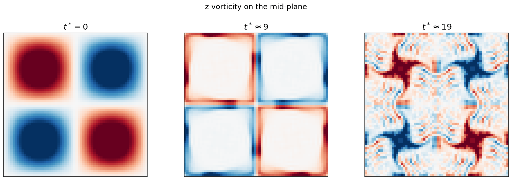
The mid-plane cuts written by the surface probe land in surface_probe/ as VTK files (view them in ParaView, or post-process them in Python). The z-vorticity on the mid-plane shows the smooth initial vortex array breaking down into small-scale turbulence:
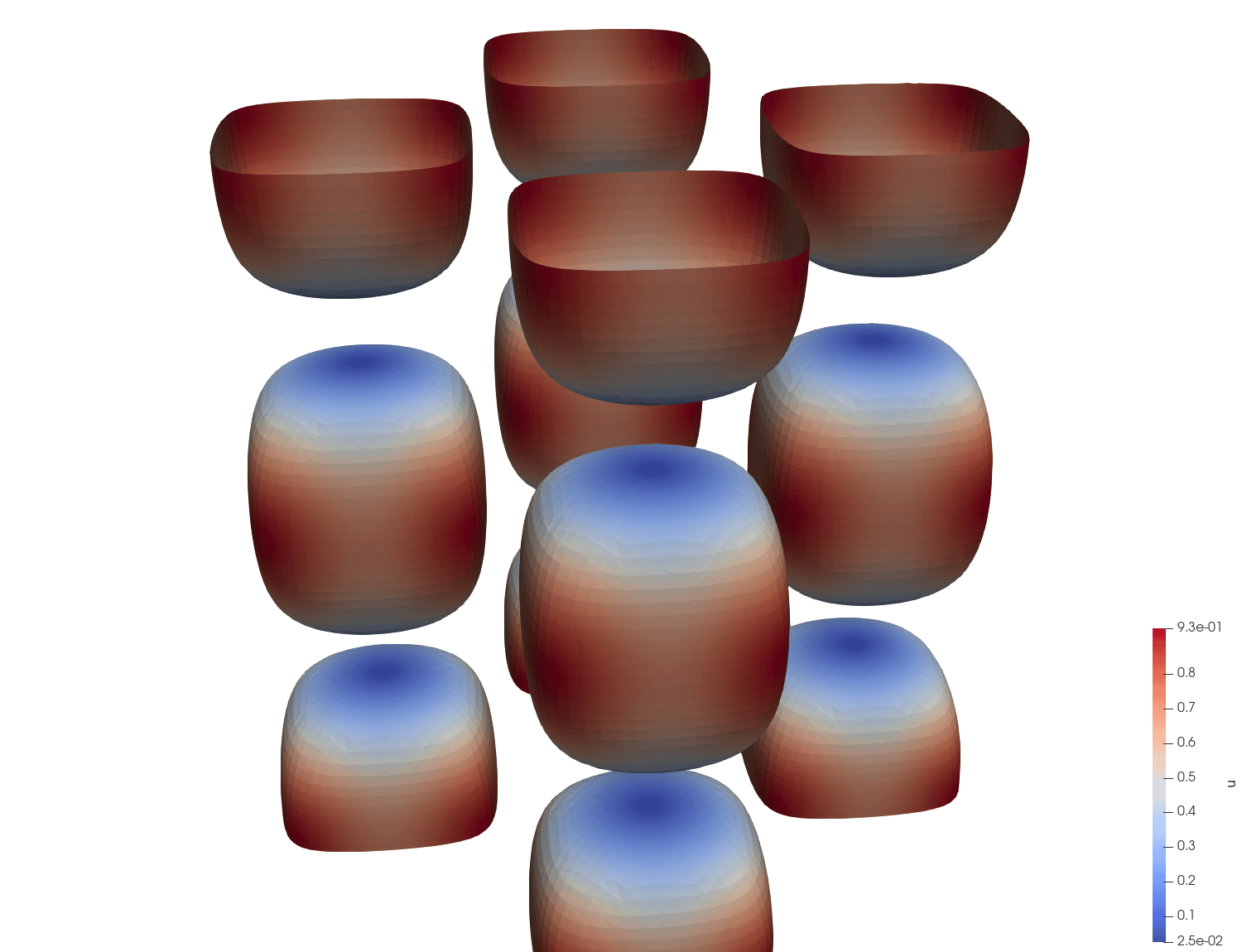
The isosurfaces_1 block extracts a Q-criterion iso-surface in situ (also as VTK, into isosurface/). At \(t^* = 0\) it shows the smooth initial vortex structure — later snapshots show it rolling up into the dense tangle of worm vortices behind the dissipation peak:
You now have a running LAVA Cartesian setup. From here:
- add refinement regions and adaptive meshing: Block-Structured Octree Meshing
- the full input reference: General Setup, Boundary Conditions, Output and Probes
- cases with geometry: the Diamond Airfoil tutorial