Running Steady-State RANS
To run this tutorial yourself, the connectivity
tutorial must first be completed to
generate the grid.x.ihc, INTOUT, grid.bc, grid.x.b2b, and
overlapper/panel_weights.dat files required as in input to the solver, or
they can be downloaded from that tutorial directly.
Navigate to the run sub-directory containing your connected grid and prepare the
files needed to run the solver by running the init_RANS.sh script, shown
below, to make a solution sub directory, then copy over and alter the input and
job submission files into it. Remember to ensure your charge GROUP_ID is
properly set in the envVars.sh file.
# Just copy over the input and pbs file, setting charge group id.
# ---------------------------------------------------------------------------- #
baseDir=$( cd -- "$( dirname -- "${BASH_SOURCE[0]}" )" &> /dev/null && pwd )

source $baseDir/envVars.sh

mkdir -p soln_RANS
cd       soln_RANS

cp $baseDir/auxFiles/LAVA_solver_RANS.yaml .
cp $baseDir/auxFiles/LAVA_solver_RANS_athena.pbs .

sed -i "#PBS -W/c\\#PBS -W group_list=$GROUP_ID" \
       LAVA_solver_RANS_athena.pbs
# ---------------------------------------------------------------------------- #
To run the solver process on the grid on a local environment, run the
run_RANS.sh script from the current sub directory. Make sure that
LAVA_EXE_DIR, LAVA_EXE_SUFFIX, OMP_NUM_THREADS, and N_PROC are properly
set in the envVars.sh file. Running with 1 MPI rank with 55 threads takes
roughly 66 minutes.
To run the solver on the NAS environment, push the following files up to
the appropriate mirrored run sub-directory on NAS if you have not
built/connected your grid there already, ssh into athfe01, cd into
soln_RANS and submit the pbs job with qsub LAVA_solver_RANS_athena.pbs,
which should take roughly 20 minutes to complete after the job begins:
grid.x.ihcgrid.bcgrid.x.b2bINTOUToverlappersoln_RANS
Input File
Below is the RANS input file in its entirety for reference, with best practice settings for transonic RANS. Specifics are discussed below.
grid :
  curv :
    gridFile :   ../grid.x.ihc
    bcfile :     ../grid.bc
    b2bfile :    ../grid.x.b2b
    fileType :   plot3d
    interpFile : ../INTOUT

timeStepping :
  steady : true

referenceConditions :
  pressure :     1.5422851978407425e+05
  uMag :         3.0583477205837789e+02
  temperature :  3.2204000000000002e+02
  alpha :        2.50
  beta :         0.0
  momentCenter : [3.9624, 0.0, 0.0]
  area :         1.3985484287039998e-01
  length :       1.9099530000000001e-01
  cp :           1005.00000
  gamma :        1.40000000
  slconst :      1.458e-6
  slref :        110.400000

nonlinearSolver :
  method :        implicit
  kind :          ank
  iterations :    10000
  miniterations : 100
  l2conv :        1e-8
  CFLStart :      0.1
  CFLlimit :      1000.0
  CFLlimitTur :   1000.0
  jacobianLag :   5

linearSolver :
  tolerance :        0.1
  maxTolerance :     0.5
  subspaceSize :     40
  approxViscFluxes : False
  lineSearch :       True
  jacobianType :     hybrid_frechet
  jacTypeSwitchTol : 1e-4

preconditioner :
  type :    ilu
  ilufill : 1
  subiter : 1

navierstokes :
  convective :
    type :           upwind
    riemannsolver :  modifiedroe
    schemeOrder :    2
    interporder :    3
    limiter :        koren
    lowspeedPreCon : none
  turbulencemodel :
    type :       sa
    userc :      True
    useqcr :     True
    usesacc :    False
    useSAlowRe : False
    mode :       zdesMode0

curvSolver :
  equations :               rans
  task :                    solve
  integrationweights :      overlapper
  integrationweightsdir :   ../overlapper
  verbose :                 False
  initializeboundarylayer : False
  echorestart :             False
  fixbadrecon :             True
  b2btol :                  1e-8
  metricexchange :          True

bc :
  -
    names : [fuse,wing,tail]
    type :  BCWallViscous
  -
    names : [far]
    type :  BCFarfield
  -
    names : [symm]
    type :  BCSymmetryPlane

output :
    ioProcs : 0

    restart :
      frequency : 500
      fileName :  restart

    volume :
      -
        frequency : 500
        fileName :  vol
        variables : ['pressure', 'velocityx', 'velocityy', 'velocityz', 'temperature', 'nut', 'eddyviscosityratio']
        fileType :  plot3d

    surface :
      -
        BCTypes :   [BCWallViscous]
        frequency : 500
        variables : [cp, signedcf, cfx, cfy, cfz, yplus]
        fileName :  surface

    monitor :
      variables : ['cl', 'cd', 'cmy', 'maxmach', 'maxanut']
- referenceConditions: Chosen to match the NTF scale wind tunnel model at Mach 0.8 and Reynolds number of 5 million.
- nonLinearSolver: LAVA best practice for steady state RANS is using the approximate Newton Krylov solver. The solution will be run until 8 orders of residual reduction occurs or 10,000 iterations have been solved. The CFL will begin at 0.1 and ramp up to 1000 to accelerate convergence as the residual is reduced.
- linearSolver: A Hybrid-Frechet Jacobian is used, and starts with an explicit matrix-based GMRES solver until 4 orders of residual reduction is achieved, at which point the solve method switches to matrix-free based GMRES.
- preconditioner: Incomplete U factorization with a fill level of 1.
- navierStokes:
- convective: LAVA best practice for steady-state RANS at transonic conditions is using an upwind numerical flux with a modified Roe Riemann solver and left and right state reconstructions, applying a Koren limiter.
- turbulenceModel: For the AOA of 2.5 simulated, best practice is to
apply both the rotational and QCR2000 corrections to the SA neg model.
For CRM high lift conditions, they should be turned off as together they
induce a lower lift near
clmax.
- curvSolver: RANS solver with fixBadRecon applied for non-subsonic flows to ensure left and right state reconstructions don't result in negative pressure and temperature.
- output: Most output variables are self-explanatory.
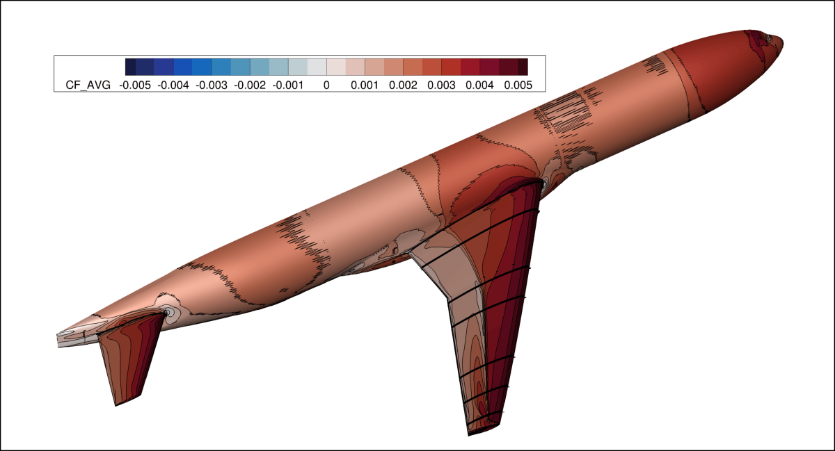
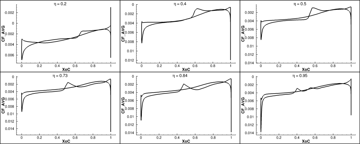
signedcfis skin friction signed using a combination of AOA and the skin friction xyz vector to showcase reverse flow regions via skin friction magnitude.
Assessing the Solution
The following files should have been written by the end of the solve, which should be pulled back to your local computer for assessment:
data.iter: the convergence history.restart.info,iter,nam,rst: files needed to restart the solver.vol.q,x,name: the last iteration's volume data.surface.q,x,name: the last iteration's surface data.
Sample shortened output from the run should look like this
                   ██╗      █████╗ ██╗   ██╗ █████╗
                   ██║     ██╔══██╗██║   ██║██╔══██╗
                   ██║     ███████║██║   ██║███████║
                   ██║     ██╔══██║╚██╗ ██╔╝██╔══██║
                   ███████╗██║  ██║ ╚████╔╝ ██║  ██║
                   ╚══════╝╚═╝  ╚═╝  ╚═══╝  ╚═╝  ╚═╝


Compiled using: Intel(R) Fortran Intel(R) 64 Compiler Classic for applications running on Intel(R) 64, Version 2021.10.0 Build 20230609_000000
  with options: -I/opt/cray/pe/mpich/8.1.33/ofi/intel/2022.1/include -I/opt/cray/pe/mpich/8.1.33/ofi/intel/2022.1/include -sox -fPIC -O3 -march=icelake-server -qopenmp -traceback -g -DLAVA_MPI
 from git hash: 63573687cd705182b4f44493e3ecae72bd21d78d*
 LAVA version : @GIT_VERSION@
            on: Aug 31 2026 at 13:04:08

 Using     4 MPI Ranks
 Using  64 OpenMP Threads

...

Proc 0 OpenMP Mapping:          Proc 1 OpenMP Mapping:
Thread:   0 Bound to CPU  0     Thread:   0 Bound to CPU 64
...
Thread:  63 Bound to CPU 63     Thread:  63 Bound to CPU127

...

--------------------------------------------------------------------------------
preprocessing
--------------------------------------------------------------------------------
readGridInfo             Time:      0.00101 seconds
setupBCInfo              Time:      0.00120 seconds
readINTOUT               Time:      0.26411 seconds
partition                Time:      0.34544 seconds
initializeTiles          Time:      0.09066 seconds
createGlobalIndex        Time:      0.27021 seconds
createGlobalVectors      Time:      0.01243 seconds
createPointHaloExchanges Time:      0.04456 seconds
createIOPartition        Time:      0.28355 seconds
readGrid                 Time:      1.35778 seconds
metric                   Time:      0.01899 seconds
setupBCsForTile          Time:      0.00945 seconds
createWallSurfaces       Time:      0.03001 seconds
createHaloExchanges      Time:      1.49440 seconds
flagNoBlending           Time:      0.00293 seconds
setupBCsForVec           Time:      0.03054 seconds
setupB2BVecScatter       Time:      0.00004 seconds
computeWallDist          Time:      3.53948 seconds
setupIntegrations        Time:      0.05246 seconds
setupTileWallIntegration Time:      0.00091 seconds
verifyB2Bs               Time:      0.06180 seconds
verifyFringes            Time:      0.00041 seconds
--------------------------------------------------------------------------------
preprocessing            Time:      8.01614 seconds
--------------------------------------------------------------------------------

...

Reference State Information:

               Reference Pressure =  154228.51978407
             Reference U Velocity =  305.54368512282
             Reference V Velocity =  0.0000000000000
             Reference W Velocity =  13.340325392204
            Reference Temperature =  322.04000000000
                   Reference UMag =  305.83477205838
                      Reference Q =  78001.073880796
         Reference Speed of Sound =  359.80561418633
            Reference Mach Number = 0.85000000000000
                  Angle of Attack =  2.5000000000000
                Reference Density =  1.6678494845492
  Reynolds Number per Unit Length =  26178654.657994
  Reynolds Number using LengthRef =  5000000.0000000
              Reference Viscosity = 0.19484819735724E-04
                     Gas Constant =  287.14285714286
             Free-Stream Residual = 0.19497029766647E+08
         Free-Stream Residual Vol = 0.41353482597890E-04
--------------------------------------------------------------------------------
--------------------------------------------------------------------------------------------------------------------------------------------------------------------------------------------------------------------------------
|     Time |Nonlin |        CFL |     CFLTur |       Wall |          Flow |           Tur | Step | Step | Step |LinIt |LinIt |Lin Res |Lin Res |            cl |            cd |           cmy |       maxmach |       maxanut |
|     Step |  Iter |            |            |       Time |           Res |           Res | Phys |   LS |  Tur | Flow |  Tur |   Flow |    Tur |               |               |               |               |               |
--------------------------------------------------------------------------------------------------------------------------------------------------------------------------------------------------------------------------------
         1       0   1.0000E-01   1.0000E-01   3.1240E+00   1.9497030E+07   6.6777235E+06  0.000  0.000  0.000      0      0   0.0000   0.0000   5.9653570E-03   7.0942371E-01   8.2683289E-02   8.5000000E-01   3.5047802E-05
         1       1   1.0000E-01   1.0000E-01   4.1014E+00   1.8906246E+07   5.5868839E+06  1.000  1.000  0.669      1      1   0.0000   0.0000   1.1358960E-02   7.0831835E-01   8.3093145E-02   8.5003932E-01   3.5047802E-05
         1       2   1.0000E-01   1.0000E-01   4.9670E+00   1.8455838E+07   4.8008919E+06  1.000  1.000  0.731      1      1   0.0000   0.0000   1.6933827E-02   7.0750977E-01   8.3546563E-02   8.5011785E-01   3.5047802E-05
         1       3   1.0000E-01   1.0000E-01   5.8332E+00   1.8110752E+07   4.2068418E+06  1.000  1.000  0.808      1      1   0.0000   0.0000   2.2706561E-02   7.0695286E-01   8.4015123E-02   8.5023461E-01   3.5047802E-05
         1       4   1.0000E-01   1.0000E-01   6.7083E+00   1.7844096E+07   3.7400436E+06  1.000  1.000  0.903      1      1   0.0000   0.0000   2.8669654E-02   7.0661139E-01   8.4480998E-02   8.5038817E-01   3.5047802E-05
         1       5   1.0000E-01   1.0000E-01   7.5762E+00   1.7633819E+07   3.3622711E+06  1.000  1.000  1.000      1      1   0.0000   0.0000   3.4794373E-02   7.0645201E-01   8.4928650E-02   8.5057697E-01   3.5047802E-05
         1       6   1.2500E-01   1.2500E-01   1.0339E+01   1.7413854E+07   2.9832121E+06  1.000  1.000  1.000      1      1   0.0000   0.0000   4.2630298E-02   7.0637965E-01   8.5419697E-02   8.5087663E-01   3.5047802E-05
         1       7   1.2500E-01   1.2500E-01   1.1206E+01   1.7247199E+07   2.6749993E+06  1.000  1.000  1.000      1      1   0.0000   0.0000   5.0501134E-02   7.0647255E-01   8.5811264E-02   8.5122546E-01   3.5047802E-05
         1       8   1.2500E-01   1.2500E-01   1.2073E+01   1.7122515E+07   2.4175369E+06  1.000  1.000  1.000      1      1   0.0000   0.0000   5.8261663E-02   7.0667434E-01   8.6104192E-02   8.5162045E-01   3.5047802E-05
         1       9   1.2500E-01   1.2500E-01   1.2942E+01   1.7030918E+07   2.1994157E+06  1.000  1.000  1.000      1      1   0.0000   0.0000   6.5797205E-02   7.0694835E-01   8.6335624E-02   8.5205882E-01   3.5047802E-05
         1      10   1.2500E-01   1.2500E-01   1.3811E+01   1.6962291E+07   2.0159631E+06  1.000  1.000  1.000      1      1   0.0000   0.0000   7.3035391E-02   7.0727535E-01   8.6563668E-02   8.5253803E-01   3.5047802E-05
...
         1     300   1.0000E+03   1.0000E+03   9.3946E+02   4.5138829E-01   5.9705310E-02  1.000  1.000  1.000     40      8   0.1542   0.0864   5.1795671E-01   2.8604070E-02  -3.8465123E-02   1.4755904E+00   3.3717311E-02
         1     301   1.0000E+03   1.0000E+03   9.4824E+02   4.6677417E-01   5.6232379E-02  1.000  1.000  1.000     34      6   0.0992   0.0889   5.1795670E-01   2.8604071E-02  -3.8465096E-02   1.4755904E+00   3.3717329E-02
         1     302   1.0000E+03   1.0000E+03   9.5633E+02   4.8309285E-01   5.5681979E-02  1.000  1.000  1.000     40      7   0.1937   0.0932   5.1795670E-01   2.8604071E-02  -3.8465074E-02   1.4755904E+00   3.3717348E-02
         1     303   1.0000E+03   1.0000E+03   9.6456E+02   5.1988277E-01   5.3544949E-02  1.000  0.800  1.000     40      8   0.1464   0.0921   5.1795670E-01   2.8604071E-02  -3.8465061E-02   1.4755904E+00   3.3717375E-02
         1     304   1.0000E+03   1.0000E+03   9.7267E+02   3.8847802E-01   4.9083825E-02  1.000  1.000  1.000     40      7   0.1287   0.0922   5.1795669E-01   2.8604071E-02  -3.8465049E-02   1.4755904E+00   3.3717396E-02
         1     305   1.0000E+03   1.0000E+03   9.8069E+02   3.7961928E-01   4.4516304E-02  1.000  1.000  1.000     40      6   0.2318   0.0974   5.1795669E-01   2.8604071E-02  -3.8465038E-02   1.4755904E+00   3.3717413E-02
         1     306   1.0000E+03   1.0000E+03   9.9060E+02   3.5494310E-01   4.2058888E-02  1.000  1.000  1.000     40      6   0.2462   0.0947   5.1795670E-01   2.8604071E-02  -3.8465035E-02   1.4755904E+00   3.3717428E-02
         1     307   1.0000E+03   1.0000E+03   9.9863E+02   3.6954132E-01   4.2434745E-02  1.000  1.000  1.000     40      6   0.2185   0.0925   5.1795669E-01   2.8604071E-02  -3.8465022E-02   1.4755904E+00   3.3717447E-02
         1     308   1.0000E+03   1.0000E+03   1.0067E+03   4.0734492E-01   4.1340448E-02  1.000  0.800  1.000     40      6   0.1659   0.0984   5.1795670E-01   2.8604072E-02  -3.8465020E-02   1.4755904E+00   3.3717465E-02
         1     309   1.0000E+03   1.0000E+03   1.0147E+03   3.1976475E-01   3.8913521E-02  1.000  1.000  1.000     40      6   0.2775   0.0920   5.1795670E-01   2.8604071E-02  -3.8465015E-02   1.4755904E+00   3.3717482E-02
         1     310   1.0000E+03   1.0000E+03   1.0227E+03   3.1172209E-01   3.6243799E-02  1.000  1.000  1.000     40      6   0.1801   0.0907   5.1795669E-01   2.8604071E-02  -3.8465007E-02   1.4755904E+00   3.3717499E-02
         1     311   1.0000E+03   1.0000E+03   1.0326E+03   3.2380852E-01   3.7397459E-02  1.000  1.000  1.000     40      6   0.1841   0.0887   5.1795669E-01   2.8604071E-02  -3.8464999E-02   1.4755904E+00   3.3717518E-02
         1     312   1.0000E+03   1.0000E+03   1.0406E+03   2.7397625E-01   3.8162284E-02  1.000  1.000  1.000     40      5   0.1002   0.0999   5.1795669E-01   2.8604071E-02  -3.8464993E-02   1.4755904E+00   3.3717534E-02
         1     313   1.0000E+03   1.0000E+03   1.0488E+03   2.2470154E-01   3.6664621E-02  1.000  1.000  1.000     40      8   0.1899   0.0976   5.1795669E-01   2.8604071E-02  -3.8464990E-02   1.4755904E+00   3.3717554E-02
         1     314   1.0000E+03   1.0000E+03   1.0571E+03   2.1174338E-01   3.3072150E-02  1.000  1.000  1.000     40      9   0.1498   0.0860   5.1795669E-01   2.8604071E-02  -3.8464987E-02   1.4755904E+00   3.3717578E-02
         1     315   1.0000E+03   1.0000E+03   1.0652E+03   1.8893928E-01   2.8632126E-02  1.000  1.000  1.000     40      8   0.1302   0.0847   5.1795669E-01   2.8604071E-02  -3.8464985E-02   1.4755904E+00   3.3717598E-02
------------------------------------------------
Info msg on proc(0) : Writing restart file...
------------------------------------------------
 solve time:   1069.52952598100       sec
  res time:   10.7660222251826       %
 form time:   3.65699977820859       %
 apply time:   29.1776649985200       %
 factor time:   5.09388768440312       %
 ortho time:   15.4056040247116       %
 turb time:   24.7732012903499       %
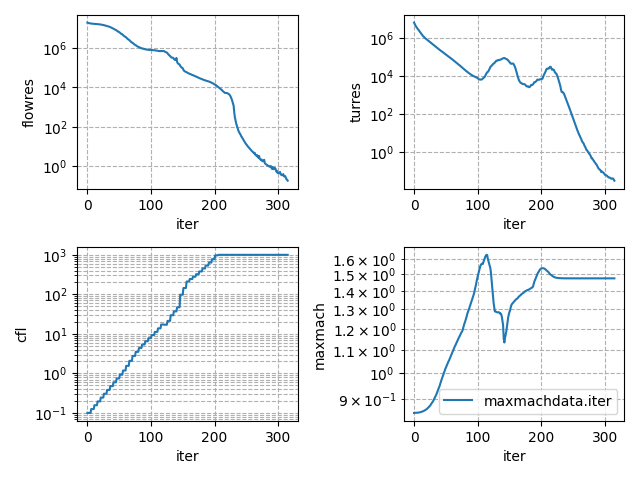
In order to monitor the residual history you can either look at the 6th and 7th
columns of the standard output which represents the L2 norm of the dimensional
flow and turbulence model residuals or you can use the plotHist plotting
utility that is provided with LAVA by running the following command
to generate the figure below which shows 7 orders of convergence within 315 iterations.
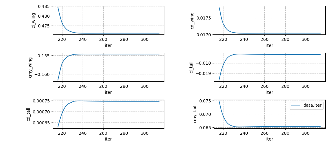
Additionally the convergence history of integrated forces and moments for the wing can be monitored by looking at the 15th, 16th, and 17th column or plotting using the following commands
plotHist.py iter cl_wing cd_wing cmy_wing cl_tail cd_tail cmy_tail -xRange 215 315 -doSubplot
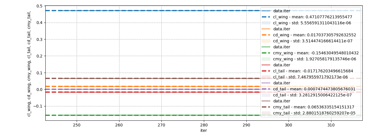
plotHist.py iter cl_wing cd_wing cmy_wing cl_tail cd_tail cmy_tail -xRange 245 315 -showStd
to generate the figures below, which show load flattening after iteration 240 and very low deviation or the last ~70 iterations.
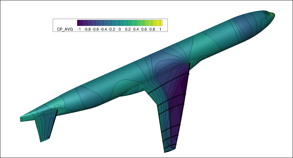
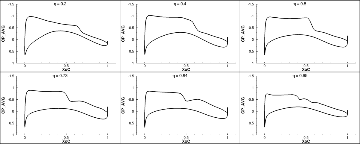
Views of the surface.q function file, surface.x grid file, and
surface.nam field name files are plotted below for average cp and skin
friction with slice plots at various slices at fractional wing span locations.
For this AOA, no reverse flow develops on the wing.