Boundary Conditions
Immersed Boundary Conditions
The LAVA Cartesian solver uses the Ghost Cell Method (GCM) for immersed boundary treatment, where ghost cells inside the body are assigned interpolated values from the fluid side to enforce boundary conditions. For details on the GCM approach, see Mittal et al.1 and for how we deal with thin geometry see Nakahashi et al.2.
Available types are: wall, inlet, outlet, nozzle,distributed, ref.
Available wall kinds are: no-slip,slip,wmpartialslip,porous,adiabatic,isothermal,wallstressmodel,musker,reichardt,blendedlog,wmnoslip,rough,roughrandom,wmslip,wmisothermal.
Available inlet kinds are: mdot,nozzle
Available outlet kinds are (optional): noreverse,dampreverse,forcesupersonic
Multiple kinds are possible for certain combinations, for example our recommended Immersed BC for WMLES:
The shorthand below is equivalent (when no velocity kind is specified,slip is assumed automatically; specifying wmpartialslip without wallstressmodel auto-adds wallstressmodel):
The available velocity treatments at an immersed wall are:
no-slip: classical Dirichlet (u = u_body) at the wall. Used for fully wall-resolved viscous simulations.slip: inviscid wall (u·n = u_body·n, tangential Neumanndu_t/dn = 0).wmpartialslip: wall-model-based partial slip. The immersed-boundary ghost-cell tangential velocity is determined by a linear reconstruction through the matching point (at off-wall distanced1) and the wall-model profile value at y⁺ =partialslipheight(default 100, deep in the log layer). This is an attempt at making the tangential velocity wall-normal gradient for the convective terms more consistent with the viscous stress correction that uses the wall function predicted wall shear stress. No wall-normal velocity is still imposed as inslip(u·n = u_body·n). When the transition sensor detects laminar flow ortau_w ≈ 0, the BC collapses tono-slip. Requireswallstressmodeland a wall-model law (blendedlogis the default).
Where, the wall stress model options include:
    # Pick wall function, kind options: musker (default), reichardts, blendedlog, rough
    kind = blendedlog
    # If using rough wall model, specify the roughness in meters
    # 0.25e-6m : highly polished
    # 0.50e-6m : polished
    # 3.33e-6m : painted
    roughness = 0.5e-6
    # Anchor y+ for wmpartialslip reconstruction (y+ units, default = 100)
    partialslipheight = 100
mdot Immersed Boundary Condition:
This boundary condition allows the user to prescribe the inflow with thermodynamic conditions, and mass flow rate. A sample setup is shown below:
  type            = inlet
  kind            = [mdot]
  mdot            = 193.1277 # Mass flow rate in kg/s
  area            = 0.162647 # Injection area in m2 (3D) or m (2D)
  #pressure        = 1e5 # Optional pressure parameter
  temperature     = 300
  massfractions   = [0.992442,1e-8,1e-8,0.007558] # If running with MS
  components      = [2] # List of components to apply this BC
pressure parameter can be prescribed to enforce a pressure along the inlet. This can be useful to model over/underexpanded inlet flows. However, for such configuration, it is recommended to use the nozzle boundary condition instead. When pressure is not prescribed, the solver will extrapolate pressure from the interior.
Info
To easily switch between 3D and 2D modes, mdot and area can be kept the same, since only their ratio is considered in the code.
Info
The thermodynamic condition description for multi-phase is slightly different than for single and multi-species. Please refer to the Cartesian Multiphase Solver page for details.
outlet Immersed Boundary Condition:
This boundary condition lets flow leave the domain through an immersed surface, such as an engine inlet face or the exit of an internal duct. The outlet surface must be a separate component of the geometry, so that the surrounding walls can keep their own boundary condition. A sample setup is shown below:
BC_1 {
  type       = wall
  kind       = [wallstressmodel,blendedlog]
  components = [1]   # walls (WMLES)
}
BC_2 {
  type       = outlet
  mach       = 0.5   # target local Mach number normal to the surface
  components = [2]   # outlet surface
}
| Parameter | Description |
|---|---|
| mach | Target local Mach number. The pressure is set from the image-point pressure by the isentropic ratio between the target Mach number and the local normal Mach number; temperature is extrapolated. Where the local flow is reversed or supersonic, a slip wall is applied instead. |
| pressure | Static pressure. Density follows from the extrapolated entropy. Ignored where the local flow is supersonic. |
| temperature | Static temperature. Pressure follows from the extrapolated entropy. Ignored where the local flow is supersonic. |
| density | Density. Pressure follows from the extrapolated entropy. Ignored where the local flow is supersonic. |
Specify only one of these. If several are given, mach takes precedence, then pressure, temperature and density. If none is given, the full state is extrapolated. Pressures are clipped to the solver's minimum and maximum limits.
The optional kinds change the treatment where the flow is reversed (entering the domain through the outlet surface) or subsonic:
noreverse: apply a slip wall where the flow is reversed.dampreverse: on reversed points, raise the boundary pressure to the isentropic total pressure for the local normal Mach number, to oppose backflow.forcesupersonic: on subsonic points, lower the boundary pressure by0.5*rho*(a - u_n)^2to drive the flow toward sonic.
The wall model is applied only to wall components with wallstressmodel; outlet components get no wall model.
Warning
- The unstructured solver's
averagemachoption (one uniform back-pressure from the area-averaged Mach number) is not available in Cartesian. Withmach, the back-pressure varies over the surface with the local Mach number; check the area-averaged Mach number and mass flow rate in your results. - With
mach, reversed points are always treated as slip walls, sodampreversehas no effect andnoreverseis redundant. This differs from the unstructured solver, which keeps the Mach-driven pressure on reversed points. - Single species only; multispecies is not supported.
nozzle Immersed Boundary Condition:
The nozzle boundary condition is mainly used for launch simulations where the boundary condition is applied to the nozzle exit. It also comes with a few physics options to improve stability and control the output. A basic boundary condition can be specified via the following:
where the nozzle boundary condition takes an input file filename which has several supported file types datafiletype described below. Like the above boundary conditions, they are applied to a component on the triangulation specified by components. In a multispecies simulation, you must also specify ispecies which corresponds to the 0 based index of the mixture in the fluid section for which species the nozzle will eject.
A complete list of all the options is provided below, along with default options where applicable:
Main Options:
| Variable | Description |
|---|---|
| filename | (Required) The filename of the describing boundary condition file |
| datafiletype | (Required) The type of datafile. 0 is a steady (constant) ascii file. 1 is radially varying constant ascii file, 2 is unsteady but constant in space ascii file, 3 is unsteady radially varying binary, 4 is unsteady radially varying ascii file |
| ispecies | (Required for multispecies/multiphase) Specifies the component of mixture for the nozzle to eject. |
| nozzlecenter | (Optional) Specifies the coordinates of the nozzle center |
| nozzlenormal | (Optional) Specifies the normal for the boundary condition to be applied on |
| radiusdirection | (Optional) Unit vector in global coordinates used for projected-radius lookup: abs((x-nozzlecenter)·radiusdirection). When omitted, the default radial distance from nozzlecenter is used. Useful for planar/slot injection profiles. |
| asciilinetimestart | (Required) Only used for datafiletype=4. Specifies the line number to start reading the file. |
| asciilinetimestop | (Required) Only used for datafiletype=4. Specifies the line number to stop reading the file. |
| asciilinetimeskip | (Optional) Only used for datafiletype=4. Specifies the stride at which to read lines from the file. Default is 1. |
| asciilinereadspecies | (Optional) Only used for datafiletype=4. Bool for whether this file contains species information as well. Default is false. |
| numberofradialpoints | (Required) Only used for datafiletype=4. Specifies the number of radial points in the file. |
Note
The mixture state prescribed when asciilinereadspecies=true takes precedent over ispecies. In this case, ispecies is disregarded by the reader.
Ramp Options:
| Variable | Description |
|---|---|
| rampsteps | (Optional) Will linearly warmup the nozzle based on rampsteps number of timesteps by taking a linear combination of the reference Q and the user specified conditions in filename. Default is 0 (no step ramping). |
| rampnton | (Optional) The timestep number to turn the ramping on. Nozzle will be off prior to this timestep. (Only used with rampsteps). Default is -1. |
| ramptimestart | (Optional) If rampsteps is not turned on, the other ramping option is using simulation time. This is the same linear warmup between ramptimestart and ramptimestop. Before ramptimestart the nozzle is off if it is specified. Default is no time ramping. |
| ramptimestop | (Optional) The simulation end time to ramping. |
| timeshift | (Optional) Timeshift can be used to shift the nozzles in time relative to the simulation time. This is compatible with ramping. Default is 0. |
Note
One should only use (rampsteps and rampnton) or (ramptimestart and ramptimestop). They will not work in a combined fashion.*
Physics Options:
| Variable | Description |
|---|---|
| multiphaseequilibrium | (Optional) Only used in cartesian + multiphase. This computes multiphase equilibrium on the boundary condition. Default is false. |
| dostagnation | (Optional) Apply stagnation inlet boundary conditions. Not supported for multiphase. Default is false. |
| doautomaticsonicinlet | (Optional) Only used when dostagnation = false. If the boundary condition goes below subsonic speed, we get pressure from the interior. This keeps the velocity at the inlet >= mach 1. Not supported for multiphase. Default is false. |
| dothroatsonicinlet | (Optional) Only used when dostagnation = true. Forces the pressure to be sonic + 1%. Not supported for multiphase. Default is false. |
Projected Radius Option (radiusdirection)
By default, nozzle profile lookup uses the geometric radius from nozzlecenter.
When radiusdirection is provided, the lookup coordinate is projected onto that direction:
r_lookup = abs((x - nozzlecenter) · radiusdirection)
This enables planar/slot style injection profiles where variation is only along one direction.
Notes:
- radiusdirection is interpreted in global/cartesian coordinates.
- The input vector is normalized internally.
- A zero-length vector is invalid and will trigger an input error.
- If omitted, behavior remains the legacy radial-distance lookup.
Example slot-style setup (vary profile along y only):
BC_1 {
    type                 = nozzle
    datafiletype         = 1
    components           = [1]
    filename             = nozzle_slot_profile.dat
    ispecies             = 0
    nozzlecenter         = [0.0, 0.0, 0.0] # Can be omitted. Solver will derive from geometry for each component
    radiusdirection      = [0.0, 1.0, 0.0]
}
ASCII Data Format
datafiletype = 0 or 1: steady, radially constant or varying, ascii file: radius(m) Pressure(Pa) Temperature(K) u_normal(m/s) u_radial(m/s)
datafiletype = 2: unsteady, radially constant, ascii file: time(s) Pressure(Pa) Temperature(K) u_normal(m/s) u_radial(m/s)
Info
Lines starting with # are omitted by the parser for datafiletype = 0, 1, 2.
datafiletype = 4: unsteady, radially varying, ascii file: line_number time(s) radius_x(m) radius_y(m) [radius_z(m)] Pressure(Pa) u_normal(m/s) u_radial(m/s) [u_azimuthal(m/s)] Temperature (m) [Species Mass Fractions]
Note
The format of datafiletype = 4 depends on the dimension of the configuration. The extra fields radius_z(m) and u_azimuthal(m/s) are required when running with 3D and must be omitted when running with 2D. Currently, the field u_azimuthal(m/s) is disregarded in the nozzle bc, however, it must still be present in the nozzle data file. Also, the fiels Species Mass Fractions are only present when asciilinereadspecies = true. Also, note that no comments are allowed in this file type format.
An example of a type-4 nozzle data base is shown below for the configuration asciilinetimestart = 0; asciilinetimestop = 30; asciilinetimeskip = 10; asciilinereadspecies = true:
  0   -10000  0.000 0 0  10000  1000   0  0    1500  0. 0. 1. 0.
  0   -10000  0.500 0 0  40000  1000   0  0    1500  0. 0. 1. 0.
  0   -10000  1.000 0 0  80000  1000   0  0    1500  0. 0. 1. 0.
  0   -10000  1.965 0 0 110000  1000   0  0    1500  0. 0. 1. 0.
  10   1.000  0.000 0 0  10000  1000   0  0    1500  0. 0. 1. 0.
  10   1.000  0.500 0 0  40000  1000   0  0    1500  0. 0. 1. 0.
  10   1.000  1.000 0 0  80000  1000   0  0    1500  0. 0. 1. 0.
  10   1.000  1.965 0 0 110000  1000   0  0    1500  0. 0. 1. 0.
  20   10000  0.000 0 0  10000  1000   0  0    1500  0. 0. 1. 0.
  20   10000  0.500 0 0  40000  1000   0  0    1500  0. 0. 1. 0.
  20   10000  1.000 0 0  80000  1000   0  0    1500  0. 0. 1. 0.
  20   10000  1.965 0 0 110000  1000   0  0    1500  0. 0. 1. 0.
  30   20000  0.000 0 0  10000  1000   0  0    1500  0. 0. 1. 0.
  30   20000  0.500 0 0  40000  1000   0  0    1500  0. 0. 1. 0.
  30   20000  1.000 0 0  80000  1000   0  0    1500  0. 0. 1. 0.
  30   20000  1.965 0 0 110000  1000   0  0    1500  0. 0. 1. 0.
Domain Boundary Conditions
Absent user inputs, the farfield domain boundary conditions are set automatically based on reference conditions (e.g. Reynolds, Mach, temperature, alpha, beta).
We recommend using the automatically generated farfield boundary conditions for most external flow cases, when used with typical CFD best practices (domain should extend 50-100 body lengths in each direction).
However, for internal flows or half-span models, it may be necessary to specify farfield boundary conditions manually.
The 6 domain face boundary conditions are specified as follows, where type and kind are given. Each entry in the arrays corresponds to the x, y, and z directions respectively (index 0, 1, 2). The lo arrays define the boundary condition on the minimum face of each direction, and hi on the maximum face.
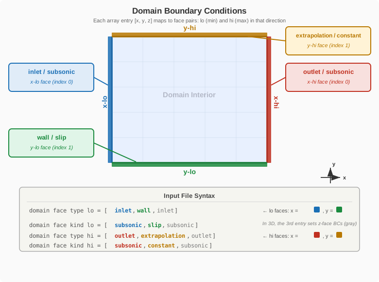
domain face type lo = [inlet    ,wall         , inlet]
domain face kind lo = [subsonic ,slip         , subsonic]
domain face type hi = [outlet   ,extrapolation, outlet]
domain face kind hi = [subsonic ,constant     , subsonic]
inlet, wall, outlet, extrapolation, ref, periodic.
Available inlet kinds are: subsonic,mdot
Available wall kinds are: no-slip,slip
Available outlet kinds are: subsonic
Available extrap kinds are: constant,linear
For half-span models, the equivalent mirror boundary condition type is wall with kind slip. Periodic boundary conditions are supported but not recommended for thin strips of airfoils or wings because it severely limits the ability to coarsen away from the airfoil: due to its forest of octree design, we currently require at least 3 boxes across the smallest domain direction on the coarsest level. If thin periodic airfoils/wings is your primary use case, we suggest using LAVACurv or LAVAUnst as they are better suited to this type of task.
-
R. Mittal, H. Dong, M. Bozkurttas, F. M. Najjar, A. Vargas, and A. von Loebbecke, "A versatile sharp interface immersed boundary method for incompressible flows with complex boundaries," Journal of Computational Physics, vol. 227, pp. 4825–4852, 2008. ↩
-
Nakahashi, Kazuhiro. "Immersed boundary method for compressible Euler equations in the building-cube method." 20th aiaa computational fluid dynamics conference. 2011. ↩