Connecting a Grid
Overset grids need to have their non-BC, or fringe, block sides interpolate from other overlapping block cells (donors) which aren't themselves near a fringe. The connectivity task within the LAVA curvilinear solver handles this donor interpolation calculation, along with many other useful data such as portions of the grid which can be blanked (removed) because of redundant overlapping of grids. Its manual can be found in the curvilinear documentation, and contains an overview of overset grid requirements, walkthrough of the connectivity process for user understanding, overview of connectivity's options in the context of the connectivity process, and a trouble-shooting section to help remove orphans (fringe nodes which can't find a donor).
To run this tutorial yourself the project grid scripting
tutorial must first be completed to generate
the grid.x and grid.bc files required as input to connectivity, or they can
be downloaded directly from that tutorial. Here we will be using the
connectivity pre-processing task to generate the following files, which can
also be directly downloaded by clicking on them here in case you can't or don't
want to run this tutorial:
- grid.x.ihc : the grid with blanking included.
- INTOUT : the fringe/donor interpolation information.
- grid.x.b2b : the block-to-block information if non-BC block faces are incident instead of overlapping.
- panel_weights.dat
: the fractional weights of each wall-surface face on the geometry which
determines its contribution to integrated values (such as loads). Note that
if you download this, put it into a subdirectory named
overlapper.
The b2b file will be calculated using the B2BExtractor utility which can be optionally triggered as a LAVA curvilinear input yaml entry, while the panel weights will be found using LAVA's overlapper utility.
Perform Connectivity
Before running connectivity, copy over and alter the needed files by running
the init_connectivity.sh script from the case directory created in the
project grid scripting tutorial.
To run the connectivity process on the grid on a local environment, run the
run_connectivity.sh script from the case directory created in the project
grid scripting tutorial to call the curvilinear solver executable you have
pointed to by appropriately defining LAVA_EXE_DIR, LAVA_EXE_SUFFIX, and
OMP_NUM_THREADS in the envVars.sh file. Running connectivity with 55
threads takes roughly 5.5 seconds with this grid, which has zero orphans.
To run connectivity on the NAS environment, submit the
LAVA_connectivity_sky_ele.pbs job. Remember to ensure your charge GROUP_ID
is properly set in the envVars.sh file before calling init_connectivity.sh
above. If you did not build your grid on the NAS system, remember to copy the
grid.x, grid.bc, LAVA_connectivity.yaml, and
LAVA_connectivity_sky_ele.pbs files into an appropriate folder on NAS and
submit the PBS script.
Input File
The connectivity yaml file is shown below. The B2B generation has been declared
using the B2BExtractor functionality. The BCs are defined with a location,
which can be onBody or offBody. Connectivity will use this information to
understand which BCs should be interpreted as part of the closed body; the
fuse, wing and tail for this case.
grid :
  curv :
    gridFile : grid.x
    bcfile :   grid.bc
    fileType : plot3d

curvSolver :
  task : connectivity

B2BExtractor :
  extractB2Bs : true

overset :
  zoneSpecific:
   -
     # All non-nose or collar near-body zones.
     zones :    [1,9-22,29-40]
     priority : 100.0
   -
     # All nose and collar near-body zones.
     zones :    [2,3-8,23-28]
     priority : 1000.0

bc :
  -
    names :    [fuse,wing,tail]
    type :     BCWallViscous
    location : onbody
  -
    names :          [symm]
    type :           BCSymmetryPlane
    location :       offbody
    symplaneorigin : [0.0, 0.0, 0.0]
    symplanenormal : [0.0, 1.0, 0.0]
    projectnodes :   true
  -
    names :    [far]
    type :     BCfarfield
    location : offbody
Output
The implicit hole cutting routines handle all geometry IO blanking well for this geometry's grid, without any user-required intervention to remove ambiguity. If portions of the geometry were disappearing or orphans existed, it may have been necessary to employ explicit hole cutters (EHCs). If simple geometry shapes were desired they can simply be put into the yaml above. As per the discussions in the project grid scripting tutorial, more component-specific cutters should be defined in that component's geom subdirectory, and then copied in and appropriately manipulated for build parameters such as yaw, etc, within the *.cut.tcl script of that component. They would then be utilized in the connectivity yaml and assigned what grids to cut by how much. For most grids no such manual intervention is required: see the connectivity manual for a larger discussion on solving orphan-related issues.
You will also note that a smallGapDetectionInfo.txt file was written. The
surface geometry must be resolved by the octree for IO testing. If the octree
is too coarse then IO tests may not be trustworthy, and this written file
states how fine the octree levels would need to be for each grid to be
completely resolved. In the case where many orphans are appearing in certain
grids, you may want to use this to identify a more reasonable octree resolution
to be assigned locally. Otherwise, it can be ignored.
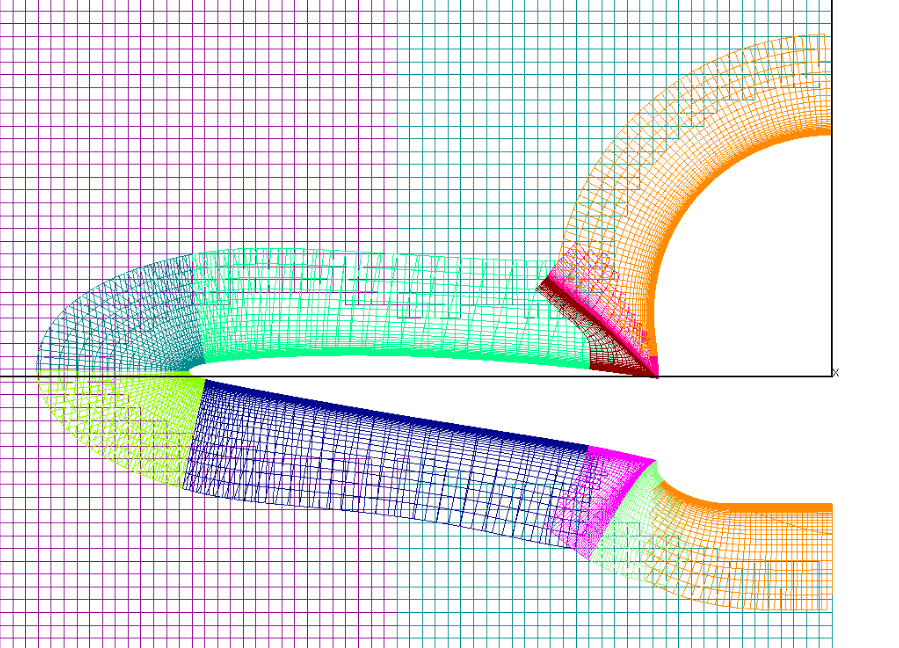
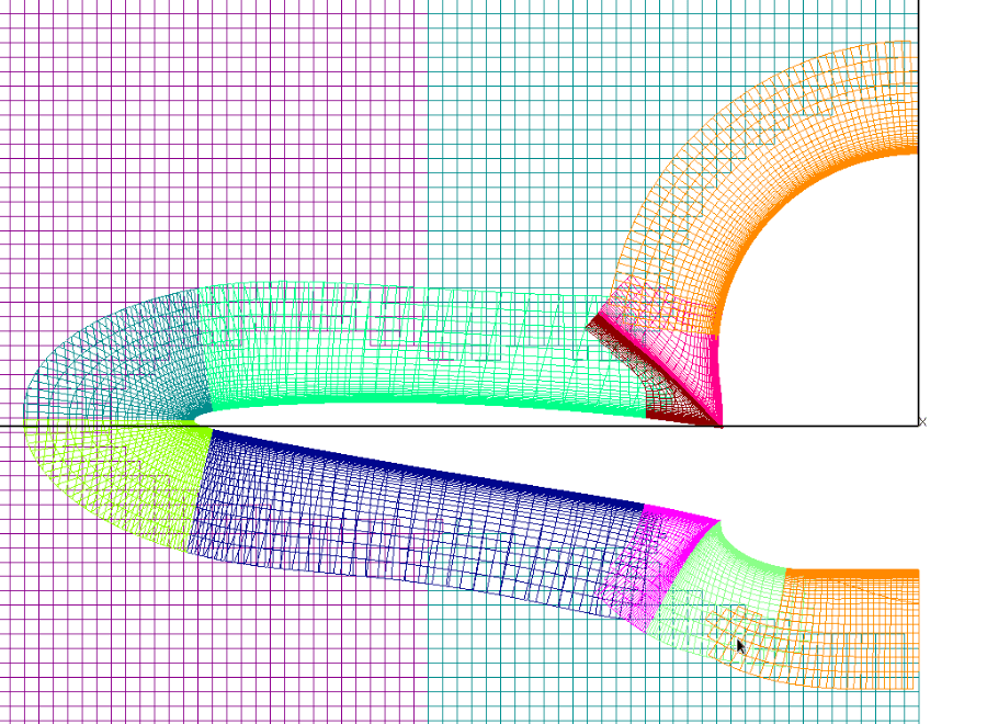
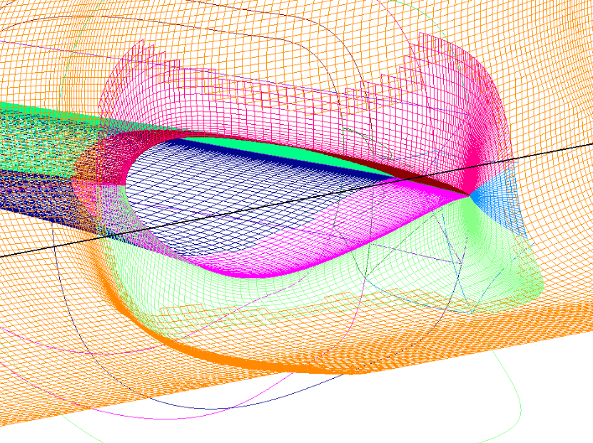
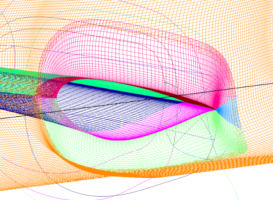
Grid Priorities
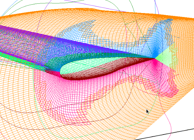
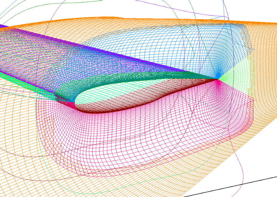
The yaml above also has a set of zone-specific commands which increase the
priority for different sets of nearbody grids. This value increases the seen
quality of those grids' nodes, forcing them to exist where other, smaller
cells would normally overtake them. Below are a series of figures with the
priority assignment removed from the yaml on the left, and included on the
right. The purpose of assigning these priorities is mainly to force the collar
grids to be retained, thus getting more consistent hole cuts with increasing
mesh resolution. You will note that the priorities do not affect how far the
nearbody grids overlap with the far-field grids: the size of the far-field cell
size local to the body in conjunction with the distance the nearbody grids are
grown out turns out to require the full nearbody grid necessary pretty much
everywhere and thus its retraction is insensitive to priority. This will change
for refined grids where more overlap exists.