Cart3D->Running flowCart

Input/Output files:

flowCart requires an input.cntl file, a mesh, and a Mesh.c3d.Info file to get running. If you want to map the solution back to the surface triangulation, then you'll also need to provide the configuration triangulation file which you used to create the mesh (in cubes). Meshes can be any one of the following:

File type - default name Contents Platform and solution approach

     Mesh.c3d Unordered mesh from cubes Single CPU, no multigrid or grid sequencing

     Mesh.R.c3d Reordered mesh ready for partitioning Multiple CPU, no multigrid or grid sequencing

     Mesh.mg.c3d Reordered, multilevel mesh file Multiple CPU, with multigrid or grid sequencing

Most often, you're feeding flowCart a "Mesh.mg.c3d" mesh, and you can delete the other files. For more information on flowCart I/O command line options and files, click here. When using the "$__Force_Moment_Processing" section in input.cntl you will also have to have a GMP-style Config.xml file, but flowCart will automatically produce one of these if the only component you're interested in is "entire".

Checkpoint files allow you to restart or reload simulations. When running steady-state they contain the current solution and are named something like check.##### where the current mg-cycle gets stamped into the #'s (e.g. check.00200). When you're running unsteady, the files get a "*.td" suffix attached to indicate that they came from a time-dependent run, (e.g. check.000200.td). You'll notice that checkpoints from unsteady runs are generally about twice as large as steady runs. This is due to the fact that unsteady checkpoints actually store two time levels worth of data. Having two time levels permit restarts to advance with full second-order time accuracy, without any hiccup in convergence. Finally, note that flowCart automatically identifies steady state and time dependent checkpoints. You can initialize an unsteady simulation from a steady state run, or even restart a time dependent run in steady state mode. Feel free to mix-and-match. MPI and Shared Memory version of flowCart are 100% compatible.

Notable new features:

Here is a short list of some notable giving you control over how flowCart/mpix_flowCart behaves and what you can make it do.

‐nSteps %d: You can now run unsteady (time-dependent) simulations. When running unsteady, we use a dual-time approach, and the ‐N %d flag tells flowCart the max number of inner mg-cycles to use within a time step.
‐stats %d: Extract statistical information like averages, min's and max's, over a temporal window of your run. "Stats" work for steady-state simulations as well, where you'll obviously get iterative averages and not time-averages. In combination with ‐T, stats also produces a distribution of min's, max's and average values over the entire surface. If you've requested loadsCC.dat, ‐stats will also produce loadsCC.avg.dat with time/iteration averaged loads.
‐fine: Modifies the meaning of ‐N so that it requests a specified number of mg-cycles on the finest mesh (coarse grid mg-cycles "don't count"). The ‐fine flag also makes ‐N incremental, so it says "run this many more multigrid cycles" on restarts.
Simpler and more flexible propulsion boundary conditions along with mass-flow steering and mass flow objective functions for adaptation and design.
Mass flow monitoring: flowCart now tracks mass flow through inlets and exits specified with the SurfBC tag in input.cntl. Mass flows through these components get reported in loadsCC.dat.
Equivalent Area Sensors: Similar to extracting a pressure distribution with a lineSensor, eaSensors extract equivalent area measured along a line in the flow.
Buoyancy driven flow: Run atmospheric simulations with buoyancy by specifying the Froude number and a gravity vector in input.cntl.

Command line options and Usage:

Usage:

% flowCart -

% flowCart -
Usage: flowCart [ OPTIONS ]

Options: -- Runtime Options-- -N %d Max Number of multigrid cycles to advance-fine Do -N cycles on finest mesh (incremental if restart) <FALSE>-mg %d Number of multigrid levels-gs %d Use grid sequencing on # levels for startup (no mg) -cfl %f CFL number-tm %f Cut-cell Grad mod (1stOrd=0. -> 1.0=2ndOrd) <def: 1.0>-limiter %d 0=None, 1=BJ, 2=VanLeer, 3=SinLim, 4=VanAlbada, 5=MinLim-buffLim Buffer limiters to neighbors default: <false>-flux %d Flux function <0> (0=VanLeer, 1=VanLeer-Hanel, 2=Colella, 3=HLLC)-no_fmg No full multigrid startup(begin MG at finestLevel)-subcell Use subcell resolution on finest mesh-gr Use grads in MGrestrict (auto ON if gradEval all stages)-choice %d 1=do_mg_new, 2=jameson, 3=orig_do_mg_cycle, <def: 3>-y_is_spanwise Default assumes z_is_spanwise direction-stats %d Compute running avgs over this many cycles or timesteps -- Unsteady Run Options -- -nSteps %d Max number of unsteady time steps (triggers time-dependent run)-dt %f Non-dimensional size of physical timesteps Lref/ainf-checkptTD %d TD checkpoint every "checkptTD" timesteps <end of run>-checkptGrads Write out checkpoint files for gradients at end of run-vizTD %d Output viz files every "vizTD" timesteps <same as checkptTD> -autoDT %d Auto adjust physical timestep for roughly const. CFLphys <FALSE> -refWaveSpeed %F Reference max wave speed (with -autoDT option) <UNSET> -track %d Track error for adapt every "track" time steps <don't track>-clean Relax solution before time-stepping and reset nSteps <FALSE> -- I/O Options -- -no_ckpt Suppress checkPointing-restart Restart into any # of partitions <Restart.file>-v Verbose mode ON-T Dump surf triangulation in Tecplot format <surfName.dat>-clic Dump surf triangulation in Clic format <surfName.triq>-his Deprecated Write [history.dat,forces.dat] <now auto on>;-no_his Turn off writing history files <history.dat,forces.dat>-binaryIO Write postprocessing data in binary (plotfiles etc.) <FALSE>-i %s Input file name, default:<input.cntl>-Xcut %d Num of X=const cut planes <disjointCutPlanes.dat>-Ycut %d Num of Y=const cut planes <disjointCutPlanes.dat>-Zcut %d Num of Z=const cut planes <disjointCutPlanes.dat>-Dcut Dump tecplottable file <cutcells.dat>-version Dump version info and exit

top

Multi-processor running:

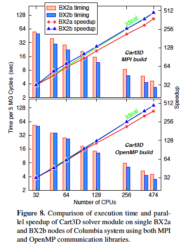
flowCart uses OpenMP or MPI for explicit communication between subdomains in multi-CPU/multi-core runs. This means that you can run it on any machine or cluster with either distributed or shared memory. Since it always explicitly decomposes the domain, both executables achieve extremely good scalability. To the right is a plot of showing parallel speedup (from Feb. 2014) for a typical case on about 57M cells.This case was run on NASA's Pleiades when it was the 11th fastest in the world. Both MPI and Shared Memory (OpenMP) versions scaling linearly down to below 100k cells per core. Here is an older comparison that was done on NASA's famous Columbia system.

More information on the programming paradigm and details of the parallelization are availible in:

‐ "Using OpenMP: Portable Shared Memory Parallel Programming" by Chapman, Jost and van der Pas. Oct. 2007
‐ "Performance of a New CFD Flow Solver using a Hybrid Programming Paradigm". Jol Para. Dist Comp. 2004 (pdf).

To run on a multi-cpu or multi-core system with OpenMP (shared memory) follow these steps (csh):

1% setenv OMP_NUM_THREADS nProc # ...nProc is the integer
#    number of CPU's you want

2% flowCart -[OPTIONS] # ...run the executable, flowCart will interrogate
#     the environment and set the number of subdomains
#     to nProc automatically

MPI executables are built using both the OpenMPI and SGI-MPT Message Passing libraries. To run on a multi-cpu or multi-core system with MPI do the following (csh):

1% mpiexec -np nProc mpix_flowCart -[OPTIONS] # ...nProc is the integer
# number of CPU's you want

Note: We frequently get questions about MPI running. mpix_flowCart is distributed using dynamically linked executables. There often turn out to be basic issues with the underlying MPI installation. If you're new to MPI, there are a couple of things you should start with before jumping in...

Run flowCart (shared memory) on more than 1 thread using OpenMP.

Does "%mpiexec -np 2 /bin/date" return 2 copies of the date?

Can you run any (other) mpi code?

Can you run any of the basic MPI demos installed on your system?

top

Flux Function Options:

flowCart is designed to allow user-selectable flux functions. Currently, van Leer, Colella'89 and HLLC (beta-test) are available. Of these van Leer ("-flux 0") and van Leer-Hänel ("-flux 1") are the most well exercised, and since they're positive flux functions, they're certain to be the most robust. Most users should choose "-flux 0" (van Leer) as their default. You can specify the flux function on the command line using "-flux 0" or by using the FluxFun tag in the $_Solver_Control_Information category of the input control file and set it to "0". Flux functions are ordered roughly in order of decreasing smearing of contact discontinuities. HLLC gets an exact contact speed, while this is the classic Achilles heel of van Leer. Take a 2D airfoil (like the naca0012 in $CART3D/cases/samples/naca0012) and experiment.

top

Robust Mode:

Starting with versions v1.3, flowCart has a new "robust mode" of operation. In general, the code is very robust running with the standard Runge-Kutta (RK) scheme sketched in the sample input.cntl file, This scheme works great most of the time, but its a compromise between robustness and speed. As is clear from the RK tags, typically you can get away with only evaluating the gradient and limiters at the first stage of the scheme, saving this work on subsequent stages. In taking this shortcut, we give up some of the remarkable positivity property of some flux-vector-splittings. By being more careful - evaluating the gradient at every stage in the RK scheme, and re-evaluating it during multigrid restrictions, the scheme can be made extremely robust.
To invoke "robust mode" simply set up your RK scheme in the input.cntl file to evaluate the gradient (and limiter) at every stage in the RK, like this:

Entries in $__Solver_Control_Information block of "input.cntl" to invoke "robust mode"

RK    0.0695      1
RK    0.1602      1
RK    0.2898      1
RK    0.5060      1
RK    1.0         1

Use "robust mode" sparingly. Nearly all calculations will run with the standard scheme (which is about 50% cheaper). Virtually all the simulations that you'll find on this website were run with the standard scheme.
top

Limiter Choice:

Starting with Cart3D_v1.3 the limiters have been completely re-coded to be better behaved than in earlier distributions. They are now linearity preserving regardless of mesh stretching, and there is a choice of 5 of them. Having said that, you should almost always use limiter 2 (van Leer). This is the most aggressive smooth limiter and is not excessively dissipative - especially in the k-exact implementation in flowCart. Furthermore, its among the fastest to compute. The limiter choices are (in order of increasing dissipation): (0) no limiter, (1) Barth-Jespersen (2) van Leer, (3) sin limiter, (4) van Albada (5) Minmod. To understand the differences between them,
Look at the figure below. The plot on the left shows the limiter value (0-1) vs. the normalized acceleration or deceleration of the data. (sketch on the left). Phi = 1 means "no limiting". The parameter f is equivalently either del+/delC or del-/delC. The Barth-Jespersen (BJ) limiter essentially follows the monotonicity boundary for a 2nd order monotone scheme, so you can think of this as an effective "upper bound" for the limiter value. More aggressive, and you're not TVD. Below this curve, and you're limiting more than is strictly necessary. All the limiters go through Phi=0 at f=0.5. This says that they recommend no limiting when the data is linear, which is necessary for a 2nd order scheme.
Relative dissipation of limiters

Basically, we have BJ as the most aggressive, and minmod as the most dissipative. Everybody else falls in between. This graph helps you understand how much dissipation you're buying when you choose something other than "-limiter 1" on the command line, or in input.cntl. About the only time you should even consider something else is for high mach number cases since the more aggressive limiters may "over compress" the shocks leading to excessive "staircasing".
Van Albada is even more dissipative, and you can see that it gives up its slope substantially more quickly than sin(). BJ, or course, holds onto its slope as long as it can without overshoots, but the transitions are abrupt.
top

How do I restart a calculation?

You can restart a calculation using the parameters in your input.cntl file, and your can override most of these, if you'd like, using command line options (preferred). Both are scanned upon restart.

1. When you run a flowCart simulation, a checkpoint file is automatically produced (you can suppress this with the "‐no_ckpt " command line option, if you know you don't want to restart). This checkpoint file is automatically named using the scheme checkpoint_file_name = check.[nCycles], so if you ran 150 cycles the restart file would be named "check.00150". When you're running unsteady, the files get a "*.td" suffix attached to indicate that they came from a time-dependent run, (e.g. check.000200.td). You can use these files to restart the calculation by soft-linking the special name "Restart.file" to the checkpoint file, and invoking the "‐restart " command line flag. e.g.

`%ln -s check.00150 Restart.file`	# create a softlink
`%flowCart -restart -N 200`	# run flowCart an additional 50 cycles

2. flowCart automatically identifies steady state and time dependent checkpoints. You can initialize an unsteady simulation from a steady state run, or even restart a time dependent run in steady state mode. Feel free to mix-and-match. MPI and Shared Memory version of flowCart are 100% compatible.

top

last update December, 2024.