|
|
Overview
 What is flowCart?
What kind of discretization does it
use?
How is flowCart integrated into the
Cart3D?
How can I extract force and moment
data? What's CLiC?
Parallelization and Domain
Decomposition
Multigrid
What is flowCart?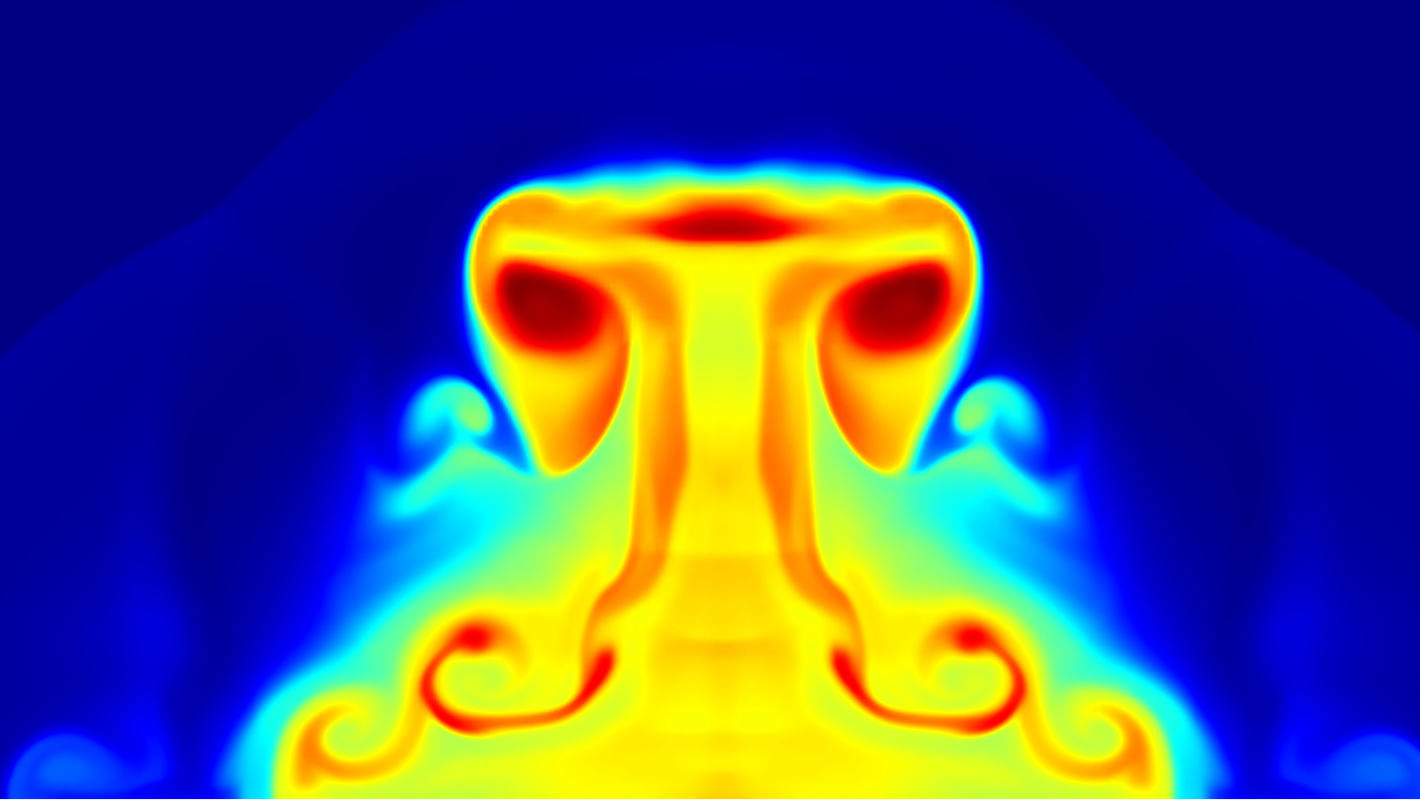
flowCart is a scalable,
multilevel, solver for the Euler equations
governing the inviscid flow of a compressible
fluid. Meshes from cubes are treated as
unstructured collections of Cartesian cells, and
it takes advantage of the fact that cells are
Cartesian wherever possible to reduce the
operation count. Both the parallelization and
multigrid are completely transparent to the user
and are turned on by simple command line arguments
to encourage their use. OpenMP and MPI versions of flowCart use
the same command line arguments, and scale
similarly.
(top)
What kind of
discretization does it use?
Spatial Discretization:
flowCart uses cell-centered,
finite-volume, upwind differencing. There are
several flux functions provided, and it is
extensible, so that you can add your favorite to
the growing list of available flux functions.
The linear reconstruction scheme makes it
formally second-order accurate, and great pains
have been taken to ensure that this accuracy is
preserved through mesh refinement boundaries and
in the arbitrarily shaped cells that appear
against geometric boundaries.
The stencil for the gradient reconstruction is
central difference, and the flux is upwind.
Implementationally, the gradient is computed
using a least-squares reconstruction, and the
least squares problem is solved via the normal
equations. At cut-cells, and cells which
neighbor refinement boundaries, the
reconstruction is always performed using true
cell and face centroids. This reconstruction is
linearity preserving, even where the mesh is
extremely non-uniform. This results in
substantially improved accuracy at
wall-boundaries and through refinement
interfaces. Results with this solver
are comparable with body-fitted structured and
unstructured solvers for comparable numbers of
cells. Most users with experience in other
packages notice that flowCart has substantially
improved wave propagation, and very low
dissipation.
Temporal
Discretization:
Steady-State
runs: Advance to steady state
is performed by an unstructured, nested multigrid procedure.
A user selectable Runge-Kutta scheme provides
inner smoothing to drive
the multigrid for rapid convergence. Virtually
any explicit Runge-Kutta
scheme can be used by putting in your favorite
coefficients (here).
Since it uses perfectly nested meshes, Multigrid
performance is competitive with better schemes
found in the literature and is really easy
to use. Of course, if you just want to
drive your solutions with plain old Runge-Kutta,
you can do that too.
Time-Dependent runs:
When
running time-dependent simulations, the
steady-state multigrid scheme becomes the
inner-driver for an outer Backward Euler (BE1)
or 2nd-Order Backward (BDF2) time-accurate
method using a dual-time formulation. Within
each time-step the multigrid converges modified
residuals using pseudo-time iterations. BDF2 is
unconditionally stable so you are free to choose
as large a timestep as your physics will let you
get away with. Unsteady restarts are
second-order in time.
(top)
How is
flowCart integrated into the Cart3D package?
flowCart
is tightly integrated into Cart3D. Pre/Post
processing operations have been substantially
reduced. Since it was written specifically as a
module for Cart3D, file translation steps have been
completely eliminated. The cubes mesh
generator puts out Mesh.c3d files, and these can be
used directly by flowCart, without translation.
flowCart can be asked to extract Cp's and other flow
quantities both on the body's surface and on cutting
planes through the domain directly (-T
and -clic
options). It also
provides both residual and lift/drag information for
convergence monitoring (the -his
option). After a run, you
can extract a variety of information using clic.
Loads and moment information are all conservatively
transferred back to the input surface triangulation,
so that you can postprocess on the surface without
having to load the entire discrete solution.
(top)
How can I extract force and moment data?
What's CLiC?
- CLiC is a
Component based force and moment module developed
as a post-processor and data-extractor for Cart3D.
Its an extremely flexible and powerful package.
Using clic, you can extract Cp cuts on any
component or group of components in your
configuration, you can compute LDM (lift, drag,
moment) for components, component groups or
configurations, and extract the usual bevy of
point-moments, line-moments ("hinge moments")
etc.. If you want to see some of what it was
designed to do, take a look at the original ISO
software project plan (here,
64kb acrobat format). Clic can be run as a
postprocessor, or called directly through an API.
The clic home page
will get you started with the package.
- You can
also automatically
extract component-based loads information
from within flowCart. Additionally, you can also
instrument your domain with point and line
sensors and collect data along these sensors
wither on-the-fly or automatically at run's end.
In v1.5 we introduced the capability to take
on-the-fly temporal (or iterative) statistics.
This includes computing average loads information
(loadsCC.avg.dat along side loadsCC.dat)
over your monitoring window. You can also extract
the envelope
and averages of local surface quantities,
so you can pinpoint which parts of a surface
geometry are most affected by local unsteadiness.
(top)
Parallelization and Domain
Decomposition
flowCart
uses a domain decomposition approach to
parallelization. As a result, scalability on large
numbers of processors is quite good. Scalability is
linear down to about 10k cells per core (2013-era
hardware) even with multigrid. In domain
decomposition approaches, the computation proceeds
on subdomains that are farmed off to the machine's
processors. After a certain amount of work is done,
each subdomain passes information to its neighboring
subdomain in an explicitly coded communication step.
OpenMP
flowCart was developed using the
OpenMP
standard. However, it is setup like a
distributed memory code, in that it uses domain
decomposition, and memory locality is carefully
controlled.
Thus, although it uses explicit message passing
and achieves excellent scalability, it is a shared
memory code. For machines with physically
distributed memory, use the distributed variant mpix_flowCart.
MPI
mpix_flowCart
was completely re-worked in Cart3D v1.5.
in v1.6 it remains 100%
feature-complete and performs all the same tricks
as the shared memory version. The code base has
been reworked for maintainability and the MPI and
OpenMP builds use as much of the same code as
possible. Scalability of the MPI code is
as good or better than the shared memory version.
Here is a comparison.
We include distributions using a variety of MPI
backends, including OpenMPI and MPICH. For a full
list of backends, see the release notes that come
with Cart3D, or look in $CART3D/bin/$CART3D_ARCH/
Domain Decomposition
Our domain
decomposition approach was designed to be
transparent to the user. It relies on a
space-filling-curve based reordering of the cubes
mesh which is then partitioned on the fly when you
startup the solver. All you need to know is that
if you want to run in parallel you just have to
(1) reorder the mesh with the reorder
utility, and (2) set your OMP_NUM_THREADS
environment variable to the desired number of
processors, flowCart does everything
else. Here's how
you'd do that for a 16 CPU case using OpenMP, (in
csh):
| 1.%
reorder |
# reorder the mesh (using
default file names) |
| 2.%
setenv OMP_NUM_THREADS 16 |
# choose number of processors |
| 3.%
flowCart |
# start the run |
With MPI,
the procedure is basically the same, but you
use mpiexec
to start the solver:
| 1.%
reorder |
# reorder the mesh
(using default file names) |
2.%
mpiexec -np 16 mpix_flowCart
|
# use
mpirun/mpiexec to set num. of processors
and run
|
(top)
Multigrid
flowCart
uses Full Approximation Storage (FAS) multigrid for
convergence acceleration. You invoke it via the
-mg %d command
line option (e.g. for 4 levels of multigrid you'd
type "% flowCart -mg 4"). By default its set up to
do use a full multigrid startup procedure. This
means that computation starts on the coarsest mesh,
once that converges a bit, the next finer mesh gets
into the act and it does two level multigrid. After
a while the evolving solution gets transferred to
the next finest mesh, and it does three level
multigrid. This continues until we've reached the
finest mesh, and then the entire mesh hierarchy is
used to converge the solution on the finest mesh.
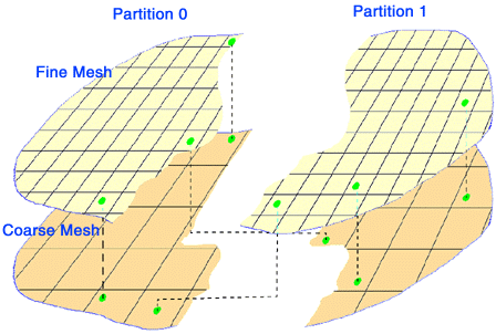
When you run in parallel, each processor gets its
own hierarchy of fine to coarse meshes to work with,
here is what it would look like for 2 processors:
Multigrid
obviously needs a sequence of coarse meshes to get
going. These meshes are derived from the fine grid
that you make with cubes. We use a special
coarsening procedure which attempts to coarsen
with an 8:1 coarsening ratio. Anytime a parent
cell finds all its children at the same level of
refinement, that parent cell gets inserted into
the coarse mesh. Of course there are situations
where one or more children has further
subdivision, and coarsening gets "suspended" in
that cell. As a result, coarsening ratios with
this algorithm approach (but do not
exceed) 8:1. In practice, finer meshes achieve
coarsening ratios above 7:1, which is sufficient
to ensure good smoothing. W-cycle multigrid
requires at least 4:1 to maintain its
(theoretical) constant time bound. Meshes at any
level in the hierarchy fully cover the
computational domain, and may contain cells at
many levels of refinement.
The mgPrep
utility takes a reordered fine mesh
(output from reorder)
and creates a sequence of coarse meshes directly
from this mesh. Since the fine mesh has already
been reordered, the coarse meshes will
automatically be ready for domain-decomposition,
should you wish to run the final multigrid run in
parallel. When a multigrid mesh is run in
parallel, all meshes in the hierarchy get
automatically partitioned using the exact same
space-filling-curves, so coarse meshes in a given
partition overlaps maximally with the finer grids
that it supports.
Building
coarse meshes with mgPrep is extremely
easy. mgPrep takes in a reordered mesh
(usually called Mesh.R.c3d) and outputs the input
mesh, and the series of coarse meshes generated.
The hierarchy of meshes is stored in a single
file, usually called Mesh.mg.c3d. Here's how (starting from
Mesh.c3d output
from cubes):
| 1.%
reorder |
#
reorder the mesh (using default file
names) |
| 2.%
mgPrep -n 6 |
#
generate coarser meshes (orig + 5
coarser) |
| 3.%
setenv OMP_NUM_THREADS 16 |
#
choose number of processors |
| 4
% flowCart -mg 6 |
# run
on 16 CPU's with 6 level multigrid |
Note: This example has some
options that you could play with, for example,
step 2 creates 5 levels of coarser meshes (with
the original mesh this makes 6 meshes total). By
default it creates Mesh.mg.c3d. flowCart's
input control file
now needs to point to this file as the input mesh.
In step 3, the example uses all 6 meshes in the
hierarchy, but you don't need to, you could use
anywhere from 1 to 6 levels of mesh, so running on
3 meshes (for example) with "%
flowCart -mg 3" would be an equally valid
command line. Even running single mesh "%
flowCart" will
work fine (in this case, -mg 1, is the default).
(top)
|
|