This section covers the operational aspects of the PEGASUS software, including step-by-step instructions on starting a new problem and generating input, executing the code, and interpreting the output. Some hints on dealing with certain issues and problems are given. For more up-to-date information on the status of the software, including recent releases, improvments, bug fixes, known bugs, and current development, see the following:

4.1 Setting Up the Input

The following are steps that should be taken when starting a new PEGASUS problem.

1. Create a project directory.
2. Prepare the volume grids as a multi-zone, unformatted, PLOT3D grid file.
3. Optionally, prepare an OVERFLOW (Refs. 3-5) input file containing the names and the boundary conditions for each mesh.
4. Run the peg_setup script. Choose option 1, which helps prepare all files necessary to run PEGASUS 5. You will be asked for the names of the grid and, if available, the OVERFLOW input file.
5. Exit peg_setup. This will have split the volume grid file into individual volume grid files in a subdirectory named X_DIR, using the p3d2peg utility. This will also have generated a file named peg.in.raw.
6. If an OVERFLOW input file was supplied, the peg.in.raw will contain boundary condition data in the BCINP namelist. If an OVERFLOW input file was not supplied, this boundary condition information must be added to the input file.
7. If the boundary condition information was added by hand, run the utility peg_hole_surf to generate the file hcutter.g. If an OVERFLOW input file was supplied, the peg_setup script will have already performed this step.
8. The hcutter.g file is a PLOT3D grid file containing the solid surfaces of the configuration. Using a plotting package, such as PLOT3D, carefully examine hcutter.g for gaps in the geometry that may affect hole generation (See Section 4.4, Operational Hints). Modify the peg.in.raw to close any gaps in the geometry by adding additional surfaces to the list of boundary conditions in the $BCINP namelists, and use IBTYP=-1 for these additional surfaces. IBTYP=-1 denotes a solid surface which will be used by the automatic hole cutting, but which will not be excluded from the list of outer boundary surface points requiring interpolation data.
9. Once corrections have been made, rename peg.in.raw to peg.in.

1. Run PEGASUS with the command:
   pegasus5 < peg.in > peg.out

2. When PEGASUS execution has completed, the XINTOUT file will be generated, along with the PEGASUS log file. The peg.out will only contain error messages. The log file will contain a copy of all the input variables, information about which processes were executed, and the amount of execution time for each process. At the end of the log file will be a table that lists, for each mesh, the number of interpolated points, stencils, and orphans. If PEGASUS was compiled with the double precision option, the XINTOUT file will be double precision. A single precision XINTOUT file can be generated by running the XIN2sp utility code.

3. Generate a composite grid file with the peg_plot utility.

4. The restarting capability is a very powerful feature of PEGASUS 5. The restart function is modeled after the UNIX "make" utility. A new mesh or input, or a changed mesh or input will cause PEGASUS to perform only the processes that are affected by these modifications. For example, if a new mesh is to be added to the current configuration, the mesh is simply placed in the /X_DIR directory and the mesh name added to the peg.in file. When PEGASUS is executed, the appropriate processes are performed to account for the modifications that were made. This also works for changes or additions in the input file peg.in.

   The restart capability allows for an incremental buildup of the PEGASUS solution. Generally, it is effective to initially run PEGASUS with a minimal input file, possibly simply the peg.in.raw file generated by peg_setup. The first run of PEGASUS will do all of the necessary interpolations. The interpolation step should never have to be done again, unless a mesh is changed or added. Subsequent runs of PEGASUS can deal with other issues, such as manipulating the hole-cutting.

   This restart capability is also very useful when PEGASUS abnormally terminates due to a system crash or when resource limits (e.g., CPU limits) are exceeded. Since PEGASUS retains all results in its work directory for all processes that have been completed, when PEGASUS is restarted, execution begins with the process that was executing during the termination. The user in this case only needs to re-execute PEGASUS; no changes in inputs are required.
    

The MPI version of PEGASUS5 should be run using mpirun or mpiexec, depending upon the type of mpi installation. The standard input file can either be read via stdin like this:

mpiexec -np N pegasus5 < peg.i

or through a command-line argument like this:

mpiexec -np N pegasus5 -ifile peg.i

The latter form is sometimes necessary when the standard input file is large, as some implementations of mpi are not able to start running successfully with large stdin. In the above examples, N is the number of processes to be used, and must be greather than 1. The parallel implementation of pegasus5 uses a master and N-1 workers. The master performs all of the I/O, and sends each of the pegasus5 sub-processes to the workers, but does not execute any of the sub-processes. Executing with N=2 results in 1 master and 1 worker, so this will run no faster than the serial code. N=3 will use 2 workers, N=4 will use 3 workers, etc.

The MPI parallelization is performed on a coarse level, in that each pegasus subprocess is assigned one processor. The number of sub-processes is a function of the number of meshes, M. For example, there are (M-1)**2 projection sub-processes, M adt processes, (M-1)**2 interpolation sub-processes, etc. Most of the sub-processes can be run concurrently. However, for example, all adt processes must finish before the interpolation sub-processes begin; all auto_hbound processes must finish before the auto_cut processes begin, etc. The more meshes a problem has, the better the load-balancing will be and the more efficient it will be. A problem with only a few meshes will only benefit from using on the order of N=5 CPUs. The best performance obtained with pegasus5mpi version 5.1g is a factor of 12 speed-up using N=20 processors on an SGI Origin system for a 52-mesh problem. To better understand the load-balancing and execution time for a particular problem, use the peg5_plotcpu.pl utility script. This perl script reads a pegasus5 output log file and uses gnuplot to create a .pdf file containing a plot of the activity on each CPU usage versus wall-clock time.

PEGASUS uses a general purpose hole-cutting methodology that will cut good holes in the majority of cases for unmodified Chimera grid systems. However, there are situations where a user might want to use another hole-generation methodology. Or, a user might have legacy grid systems with previously generated hole definitions which have been successfully applied in the past. In those cases, it may not be necessary or desirable to use the hole-cutting methodology in PEGASUS; however, a user may still want to take advantage of other aspects of PEGASUS, such as level 2 interpolation. To accommodate these situations, a methodology has been developed whereby these externally defined hole definitions can be used within PEGASUS 5.1.
 

To use external hole definitions, a PLOT3D file with IBLANK records must be provided, with IBLANK=0 specified for each hole point. The IBLANK records may be generated by any means at the user's disposal.
 

• Run the utility code p3d2peg. The PLOT3D grid file and the mesh.list file (generated by the utility code mesh_lister) must be in the project directory. p3d2peg will ask if you want to use the existing IBLANK file for hole definition (answer in the affirmative). If p3d2peg detects grid files in the /X_DIR directory, it will ask if you want to replace them. Unless one or more grids have been modified since the last PEGASUS run, answer "no". The IBLANK records will be copied into the appropriate /WORK subdirectories.
• Edit the peg.in file to include "HCUT=.FALSE.," in the $GLOBAL input record.

• Run PEGASUS in the normal manner. If this is the first PEGASUS run, the entire interpolation process will be executed. If the interpolation process has been done earlier, the restart capability of PEGASUS will use the existing interpolation information to generate an XINTOUT file with the externally generated hole definitions.

PEGASUS 5.1 is highly automated, in the sense that much less user input is required to obtain a chimera interpolation file than was required in earlier versions of PEGASUS. However, automation generally requires making some assumptions about the input; if these assumptions are incorrect, PEGASUS may do something other than what the user expects or desires, resulting in varying degrees of user distress. One assumption is that hole cutting surfaces are watertight, in the sense that no gaps occur in the aggregate of the solid walls of the aerodynamic configuration. However, some common approaches to defining solid wall boundary conditions in flow solvers may, to PEGASUS, represent gaps which will adversely affect the generation of the Cartesian meshes that PEGASUS uses for cutting holes.

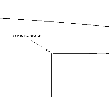
Consider, for example, the solid surface generated when the OVERFLOW input used in the 3-element airfoil example is used to generate the peg.in file using the peg_in utility code. Figure 11 depicts the region near the corner under the back of the main wing.
 

In an effort to not specify the corner point twice as a solid boundary condition, the corner point is included in the specification of the vertical surface, but not in the horizontal surface. This is fine as far as the flow solver is concerned, but PEGASUS sees this as a gap in the surface.
 

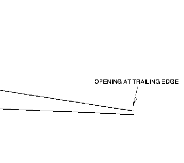
Figure 12 depicts the trailing edge of the wing. The upper and lower surfaces of the trailing edge are from two different meshes; these meshes overlap one grid point past the end of the trailing edge. Solid surface boundary conditions are specified up to the end of the trailing edge; beyond that point, the boundaries are updated via chimera interpolation. As in the corner example, PEGASUS sees a gap in the surface.
 

The effects of these gaps become apparent during the hole-cutting process. Recall from Section 2.1 that the outside region is defined by marching inward from the corners of the Cartesian mesh; any unidentified Cartesian element that is adjacent to an outside element must also be an outside element. It is clear that if the Cartesian mesh is fine enough, outside elements can "leak" through the gaps in the surface and misidentify elements inside the body as outside elements. Therefore, no hole will be cut.
 

The remedy for gaps in the surfaces depends on the nature of the openings. In the case of the corner gap, the peg.in file can simply be modified to extend the solid boundary of the horizontal surface to the corner. The trailing edge gap, however, requires the addition of another boundary surface in the $BCINP namelist, and use IBTYP=-1 for this additional surface. IBTYP=-1 denotes a solid surface which will be used by the automatic hole cutting, but which will not be excluded from the list of outer boundary surface points requiring interpolation data.

There is always a possibility that a small gap, such as that shown in the airfoil trailing edge in Figure 12. If the gap is smaller than the vertical spacing of the Cartesian mesh, the surface is closed as far as the Cartesian mesh is concerned. In some cases, the gap could be up to twice the corresponding spacing of the Cartesian mesh and still result in a good hole definition.

Other methods for fixing surfaces with gaps is with the use of auxiliary (i.e., "phantom") meshes. These meshes are designated in the standard input file in the $MESH namelist by setting PHANTOM=.TRUE. The solid surfaces of a PHANTOM mesh are to be designated in the BCINP namelist for the phantom mesh. The phantom meshes do not participate in the interpolation, and do not appear in the output XINTOUT file.

Finally, problems with automatic minimum hole cutting can be remedied with the use of the manual hole cuts, which use the hole cutting algorithm in PEGSUS 4.1. Manual hole cutting surfaces are specified using the $BOUNDARY and $SURFACE namelists.
 

4.4.2 Thin Trailing Edges
 

The hole cutting algorithm is a very general approach, and can accommodate unmodified chimera grids systems with overlapped collar grids and multiple interior regions (which occur, for example, in the 3-element airfoil example). However, modern chimera systems often have a very large size range of surface features that the Cartesian hole cutting meshes must resolve. In the case of very fine features on a large configuration, the resolution required may be excessive. Consider, for example, the trailing edge of slat in the 3-element-airfoil example. Figure 13 depicts a point inside the
 

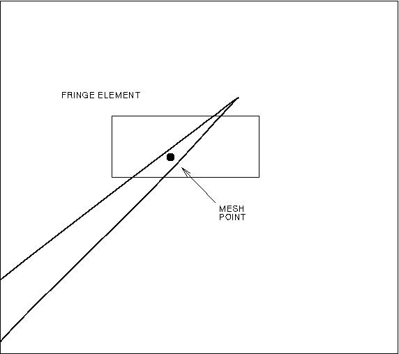
trailing edge of the slat. The solid surfaces of the trailing edge are encompassed by fringe elements, only one of which is shown for purposes of clarity. Recall from Section 2.1 that points inside fringe elements use a "line-of-sight" algorithm to determine their status. To reiterate, if a clear line-of-sight exists from a point in a fringe element to another non-fringe element, then the point adopts the status of the non-fringe element (either "outside" or "inside"). However, the point in this example may not have a clear "line-of-sight" to a non-fringe element, and therefore cannot be identified in this manner. If a point cannot be identified, it is assumed to be an outside (i.e., field) point. If the field point is next to a hole point, it will become a candidate for interpolation; being inside the slat, there will be no viable interpolation stencil, and the point will be an orphan.

Fortunately, points in thin trailing edges can often be blanked as desired using the OFFSET input in the $GLOBAL or $MESH input records. Setting OFFSET = 2, for example, grows hole regions by blanking any non-hole point within 2 indices of a hole point. In this manner points in thin trailing edges that are destined to be orphaned may be correctly blanked.

Also, multiple hole cutting groups can be used in PEGASUS. Separate hole cutters can be designated, for example, for the slat, wing, and flap separately. The Cartesian cutters are automatically sized according to the solid surfaces in the group. Specifying a separate hole cutter around the slat will automatically increase the default resolution of the Cartesian hole-cutting mesh in the region of the trailing edge. An example of input which invokes multiple hole cutters is reproduced in Appendix B. Finally, the default logical dimensions of the Cartesian hole cutter may be increased until there is sufficient mesh resolution to resolve the trailing edge.

4.4.3 Projection
  The value for DISTANCE in the $GLOBAL and $MESH namelists will control how many points can be projected. If DISTANCE is too large, it is possible for PEGASUS to project points too far, and actually move them from one component to another. It is advisable to routinely check the results of the projection by checking the maximum distance projected. This is reported in the log file, and is also easy to check by running the utility peg_proj.

In cell-center mode, the PEGASUS code treats the center of the cell volumes as the location where the flow solver will store its variables. All hole-fringe points and outer-boundary fringe points are located at cell centers. All interpolation stencils use the cell-centers from neighboring meshes to compute the stencil weights for updating these fringe cell-centers. In this mode, neighboring meshes will need more overlap to connect the cell centers compared to traditional node-based grid systems.

Take the following steps to run the code for cell-centered meshes:

1. Generate node-based volume meshes and install in the X_DIR directory.
2. Set CENTER = .TRUE. in the $GLOBAL namelist.
3. Set OUTTYPE = 2 or 3 in the $GLOBAL namelist.
4. Run the PEGASUS 5 code.
5. Use the utility peg_plot_center to generate the final grid file.
6. Use the dcintegrity utility to verify the contents of the pegasus5.dci file.

4.5.1 Cell-Centered Block Meshes The PEGASUS 5 code provides limited support of the use of overset grids together with pointwise-continuous non-overlapping block grids, also known as abutting block grids. Block grids are identified with the use of the point-wise matched block boundary, or IBTYP=20, in the $BCINP namelist. No other block connectivity information is required in the PEGASUS 5 input, the code is programmed to automatically identify the block-boundary connections on its own. Internally, PEGASUS 5 uses layer of ghost cells added to the block-boundary interfaces to enable these as donor cells to neighboring overset meshes. The code is limited to block-boundaries where one entire boundary face of one zone has exact pointwise matching to an entire boundary face of a neighbor zone. The boundary-condition of IBTYP=20 must be specified to the matching faces of both zones, and must cover the entire boundary face of both zones. In addition there is a limitation to the use of hole cutting near a block boundary. The code will not properly identify all fringes on a neighboring grid when a hole comes close to but does not intersect the neighbor block boundary. In such an instance, pegasus5 does not report an error, but the flow solver might indicate an error if it checks for fringe-point coverage across block boundaries. In this instance the best work-around is to convert the block abutting zones into overset zones by expanding/growing the grids to create an overlap.

4.5.2 Cell-Centered Indices A number of inputs require grid indices to identify points, lines, surfaces, or volume subsets of mesh. Here we identify whether specific inputs refer to the mesh cell centers or to the mesh nodes.

• $MESH namelist: the JINCLUDE, KINCLUDE, LINCLUDE indices refer to the mesh cell centers.

• $BCINP namelist: the JBCB, JBCE, KBCB, KBCE, LBCB, and LBCE indices refer to the mesh nodes.

• $SURFACE namelist: When the surface is part of a BOUNDARY namelist of type outer, the JRANGE, KRANGE, and LRANGE indices refer to the mesh cell centers. When the surface is part of a BOUNDARY namelist of type hole, the JRANGE, KRANGE, and LRANGE indices refer to the mesh nodes.

• $VOLUME namelist: When the volume is part of a REGION with TYPE=HOLE or TYPE=UNBL, the JRANGE, KRANGE, and LRANGE indices refer to the mesh nodes. When the volume is part of a REGION with TYPE=INTR, the JRANGE, KRANGE, and LRANGE indices refer to the mesh cell centers.

4.5.3 Known Problems For Cell-Centered Meshes

• The code does not always find donors for fringe cell-centers next to a wall when the overlapping meshes do not have the same wall spacing. These cell-centers are identified as orphans.

• There is a known problem in the outer-boundary stencil in a cell-center in the corner of the grid where one adjacent boundary is a multi-block boundary and the other adjacent boundary is an overset outer boundary. Part of the stencil can include itself, and the boundary might never get updated properly.

• The code currently does not level2 fringes whose donors are block-boundary ghost-cells.

• The code currently does not add outer boundary fringes to ALL cell centers in the corners adjacent to a surface with a boundary condition and an overset outer boundary.