Input Files

The default version of the aero.csh script is installed in $CART3D/bin. You should copy this template script into your run directory. Alternatively, the scripts in $CART3D/cases/samples_adapt may be even better templates. For example, if your case is 2D then a good starting point is the $CART3D/cases/samples_adapt/naca0012/aero.csh script.

The aero.csh script requires three Cart3D input files:

• wetted surface triangulation file, Components.i.tri (must be watertight)
• cubes' input file input.c3d
• flowCart's input file input.cntl augmented with a $__Design_Info section (see output functionals)

Optionally, you may also include a GMP configuration file Config.xml. The surface triangulation file must be called Components.i.tri. In practice, the surface triangulation can be called anything - just create a symbolic link to Components.i.tri. We recommend autoInputs to create input.c3d. You may also use the preSpec.c3d.cntl file to specify BBox and XLev regions for cubes (this can be useful for cases with power boundaries) and ABox regions for adapt (use cautiously, not recommended in general).

Aero.csh Parameters

The many user-adjustable parameters of aero.csh are divided into three groups: Basic, Advanced and Expert sections. All options are documented inline. Further documentation of options related to cubes and flowCart is available here. To get started, the two most important flags are mesh2d and y_is_spanwise in the Basic section. The default settings assume a 3D case:

set mesh2d = 0

and that the geometry is in a Y-is-up and Z-is-spanwise orientation:

set y_is_spanwise = 0

The default parameter values in $CART3D/bin/aero.csh are conservative - we found them to work robustly in difficult cases, e.g. cases with strong power boundary conditions. The aero.csh scripts in $CART3D/cases/samples_adapt have settings more appropriate for typical cases, such as transonic flow around transport configurations. These should give better accuracy and faster turn-around. Frequently adjusted parameters include:

• Number of refinement cycles n_adapt_cycles
• Number of multigrid levels mg_fc and mg_ad

Important parameters that influence the efficiency and accuracy of adaptive runs are the mesh-growth and adapt-propagate arrays, and the auto_growth option. These parameters are described in the Advanced Run Control section below, their defaults should be fine for getting started.

Upgrading Older aero.csh Scripts

Traditionally, it has been straightforward to migrate from older versions of aero.csh to the latest release. However, the input parameters have been significantly reorganized and modified in the 1.5 release. In an effort to make the porting easier, a utility script aero_upgrade.py is provided to automatically upgrade aero.csh. The script uses the master copy in $CART3D/bin/aero.csh as a template to port the user settings from the old version. Execute the script in the directory containing the old aero.csh:

% $CART3D/bin/aero_upgrade.py

The script leaves a backup of the original in aero.csh.orig. Always check the new script against the backup.

Usage

To run the adaptation, simply execute aero.csh:

% ./aero.csh

The script returns 0 on success and 1 if an error occurs. (Novice Linux users: the ./ means to execute the aero.csh that is in the current directory, not the one in $CART3D/bin.)

The script accepts several command line arguments. To see a usage statement use the help or -h options:

% ./aero.csh help

To restart an adaptation run, increase n_adapt_cycles and use the keyword restart as follows:

% ./aero.csh restart

The restart flag can be also used to recover from a crashed run, e.g., machine crashes. To restart from a particular adaptXX directory, delete all adapt?? directories after adaptXX and restart.

To start an adaptation run from an existing mesh, place Mesh.mg.c3d and Mesh.c3d.Info files into the run directory and use the keyword jumpstart as follows:

% ./aero.csh jumpstart

Jumpstarting is useful for restarting an adaptation form some previous adapt?? directory. Simply copy the desired mesh files to a new run directory and continue adapting. When aero.csh executes, the mesh files are moved to the adapt00 directory.

Advanced feature: at the start of each adaptation cycle, aero.csh checks for the presence of input.new.cntl file. If this file is present, it will replace the active flowCart input.cntl file. This feature allows on-the-fly control of the flow solution as the adaptation executes.

To stop an adaptation run after the computation of the next error estimate, create a STOP file:

% touch STOP

To clean-up a run directory and start a new run on the same case, remove the adapt?? directories:

% rm -rf adapt??

Setting environment variable debug_verbose (% setenv debug_verbose) triggers more verbose output.

Outputs

The file and directory tree of a typical adaptation run, with n_adapt_cycles = 2, is shown below:

naca0012
|-- ADAPT
| |-- # Generation of adapted meshes
| `-- adapt.*.out
|-- BEST@ -> adapt02
|-- EMBED
| |-- # Generation of embedded meshes
| |-- Error_in_J
| | |-- # Error estimation
| | |-- adjointErrorEst.*.out
| | `-- cutPlanesErrEst.*.plt
| `-- adapt.*.out
|-- adapt00
| |-- AD_A_J
| | |-- # Adjoint solution
| | `-- cart3d.out
| |-- FLOW
| | |-- # Flow solution
| | |-- cart3d.out
| | |-- entire.dat
| | |-- forces.dat
| | |-- functional.dat
| | |-- history.dat
| | `-- loadsCC.dat
| |-- Mesh.c3d.Info
| |-- Mesh.mg.c3d
| `-- cart3d.out
|-- adapt01
|-- adapt02
|-- aero.csh*
|-- all_outputs.dat
|-- Components.i.tri
|-- fun_con.dat
|-- input.c3d
|-- input.cntl
|-- results.dat
`-- user_time.dat

Red marks input files; not all outputs are listed. Each adaptation cycle generates a new adapt?? directory that holds the flow and adjoint solutions of the current mesh in the subdirectories FLOW and AD_A_J, respectively. The output (stdout and stderr) of the various codes that execute in these directories is directed to files called cart3d.out in the FLOW and AD_A_J subdirectories. This is a good place to look if your run has crashed and you're trying to figure out the problem. The script also maintains a link called BEST.

The BEST Link

The BEST symbolic link always points to an adapt directory that contains the best solution obtained so far. Under normal circumstances, this link points to the last adapt directory. Various conditions, such as run termination due to a machine crash or queue time expiration or solver divergence may cause an unexpected exit. The script ensures that BEST always points to a valid, best-so-far flow solution and is intended for use with automatic results-harvesting scripts.

Functional Convergence

The script generates at least two summary files: fun_con.dat and results.dat. The file fun_con.dat contains four columns: adaptation cycle, number of cells in the mesh, functional value and average functional value. The average functional value is useful for cases where the functional does not reach a steady value but instead becomes oscillatory. The avg_window variable in aero.csh can be used to specify the number of flow solver iterations to be used for functional averaging on each mesh.

The file results.dat contains nine columns:

1. Adaptation cycle
2. Number of cells in the mesh
3. Log of the number of cells (useful for formal convergence studies)
4. Functional value (should be same as in fun_con.dat)
5. Corrected functional value
6. Adaptation error estimate
7. Adaptation error estimate normalized by etol
8. Value of etol
9. Functional error estimate

Consult NASA TM-2014-218386 for a precise definition of these terms. The main idea is that as the mesh is refined, the error estimates should decrease and eventually fall below etol. This is one of the adaptation exit criteria. The run terminates after the next flow solution. There are two benefits to delaying the exit until after the flow solution. First, the approach is conservative in terms of the error estimate value - the functional on the next mesh should be well within the tolerance. Second, we have done all the hard work of computing the mesh refinement parameter so let's use it and compute the best solution possible.

Here is an output example from $CART3D/cases/samples_adapt/wing. The top-left plot shows the functional values (C_D) as the mesh is refined (column 2 versus 3 of fun_con.dat) with error bars representing the level of discretization error (column 9 of results.dat). Top-right figure shows convergence of several error estimates: the red line (squares) shows the reduction in discretization error after each adaptation, i.e., the magnitude of the error bars from the left plot, the black line (circles) is the magnitude of the adaptation error indicator (column 6 in results.dat), and the blue line is the change in C_D relative to the previous mesh. The bottom plot shows the iterative convergence of C_D for all adaptation cycles. After each warm-start, the initial transient quickly dissipates and the value of C_D levels out. This is a good check to make sure that the solver is running a sufficient number of multigrid cycles on each mesh.

We caution the user that the file-size and number of files generated by aero.csh can be considerable, especially when building databases with several thousand cases. This is done to provide a full history and restart capability of the runs. We provide an aero_archive.csh script for archiving runs, which significantly reduces storage requirements. Once executed, the restart capability is lost, but all important output files are kept. A possible implementation is to check the return code of aero.csh, and if zero then call aero_archive.csh. Alternatively, this script can be called from aero.csh by using the archive option:

% ./aero.csh archive

Mesh Growth

In each adapt cycle, the maximum number of cells added to the mesh is controlled by the mesh-growth factor. There are two ways to set the mesh growth:

1. Specify growth factors explicitly via the mesh_growth array. The factor may range from 1.01 to 8, where specifying 8 means that you allow refinement of every cell in the mesh. The basic idea is to adhere to a strict cell budget, thereby fixing the cost of the adaptive run. The way this works is that the cells are ranked from highest to lowest error and a fraction of the worst-error cells is refined such that the target mesh-growth is satisfied.
2. Allow aero.csh to automatically determine growth factors by setting auto_growth=1.

Note that aero.csh monitors max_cells2embed and automatically adjusts the mesh growth so that this cell limit is never exceeded. To request automatic growth rates only in specific cycles, set the mesh_growth to 0 (zero) in those cycles and disable global auto-growth by setting auto_growth=0.

General tips:

• In the default mesh_growth sequence, we start with smaller factors because the accuracy of flow and adjoint solutions is poor on coarse meshes. We go after cells with largest errors. The sequence is tuned to efficiently provide the "best" mesh possible for your cell budget.
• If the simulation contains regions of separated flow (poor solver convergence), you may try to keep mesh growth low to develop the mesh in the well-behaved regions first, and then increase it quickly to fill in the rest of the mesh.
• Cell-wise error distributions can be viewed by plotting the files cutPlanesErrEst.*.plt found in the EMBED directory. The cell-wise errors are extracted for the same cut-planes as the flow solution, which are specified in the $__Post_Processing section of the input.cntl file. The error cut-planes show the normalized cell errors - this means that we take the adjoint error estimate and divide it by the allowable error-per-cell. The allowable error-per-cell is simply etol divided by the number of cells in the mesh.
• Try the auto_growth option, it generally works very well. In our production runs, we frequently specify a mesh_growth of 0 in most adapt cycles, except in the final one or two cycles where we may specify a larger growth explicitly.

A/P cycles

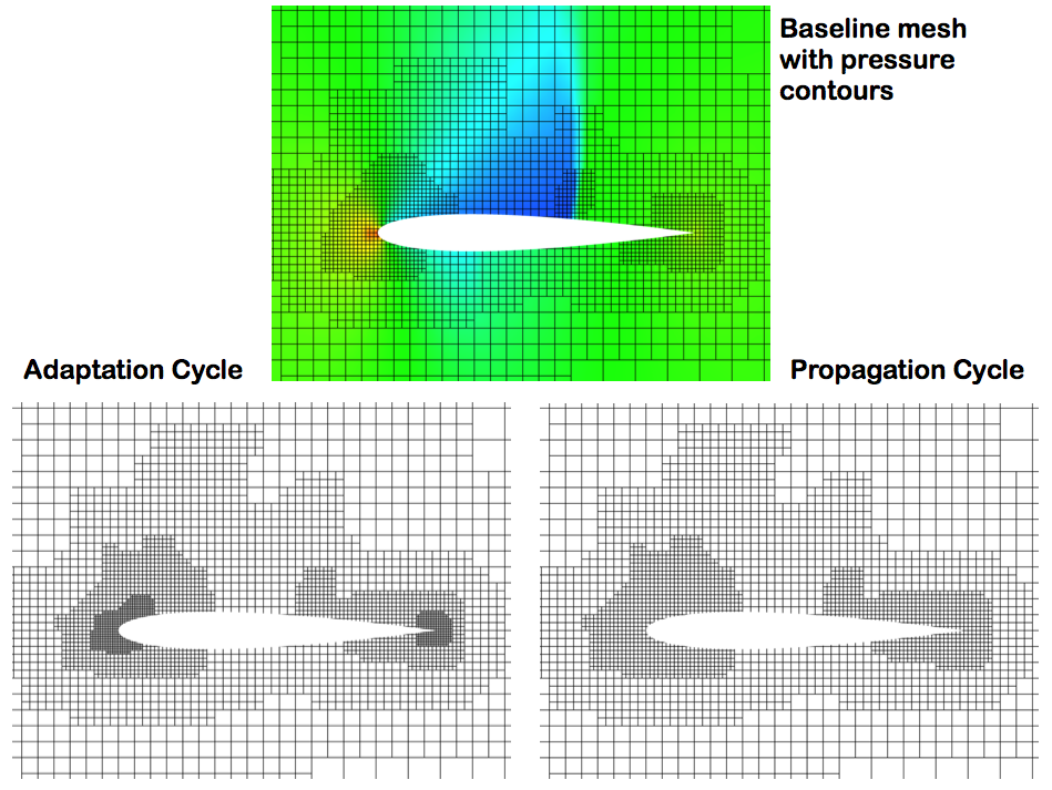
The apc array controls the refinement level of the mesh for each adaptation. It is a sequence of a and p characters that represent the following:

The purpose of a propagation cycle is to adjust cell-refinement boundaries. This is especially important in problems where the output's zone of dependence involves a large portion of the volume mesh, e.g. sonic-boom problems. Figure below shows the difference between an a and p refinement:

Tips:

• In general, use a cycles.
• We use a single p cycle on the initial mesh to reduce the bias of this mesh on the solution.
• Pay attention to the refinement level of the volume mesh relative to the size of the triangles on the geometry. In regions of high surface curvature, each Cartesian cell should be supported by several triangles. Once the size of the Cartesian cells approaches the size of the triangles, the user should switch to p cycles to prevent over-refinement of the surface triangulation. This is the best mesh you can get for a given (fixed) surface triangulation.
• Finishing the adaptation with a p cycle usually works well. This strategy prevents over-refinement of the surface triangulation mentioned above and delivers smoother meshes.

Extra Refinement Passes

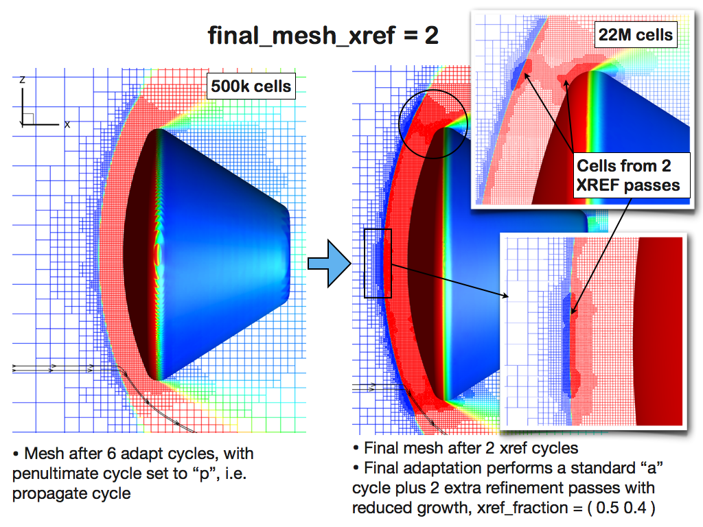
The parameter final_mesh_xref (0/1/2) allows extra refinement passes on the final mesh. When non-zero, the final error map is extrapolated to the adapted mesh such that the adaptation can be performed multiple times. This circumvents the flow, adjoint and error estimation steps, which reduces memory requirements and improves turn-around of the adaptive run. The total mesh growth is the sum of the mesh growth on the last adapt cycle plus the mesh growth in each xref iteration. This can be fine tuned via the xref_fraction array. We take the mesh growth specified for the final cycle and multiply it by the fractions specified in xref_fraction. The main idea is to focus the refinement on the highest error cells. In other words, refine regions only where the error map is most accurate.

As the error map is no longer updated to reflect the flow on the refined mesh, this is only appropriate for 1 or at most 2 refinement passes. The default value is 0 (no xrefs). In general, we obtain excellent results with final_mesh_xref=1. The figure below shows a good example with final_mesh_xref=2, where an error map that is constructed on a mesh with 500k cells is used to build a mesh with 22M cells.

(top)
(adjoint docs)