OVERSMART USER'S GUIDE

Authors: David L. Kao, William M. Chan, Chase P. Ashby

Version: 4.0

Date: September, 2025

Introduction

OVERSMART is a program that offers the user a convenient way to rapidly examine the convergence behavior of flow computations for complex configurations. Output statistics offer a concise summary of the time histories of flow variables and turbulence model residuals, and component forces and moments. Currently it is targeted for the OVERFLOW-2 flow solver but extensions can be made to allow other flow solvers.

Figure 1. An executive summary page generated by OVERSMART.

Installation

Execution of OVERSMART requires Python version 3.0 or higher. One of the following plotting packages is assumed to be installed on the user's machine:

xmGrace - this is the default plotting package to be used.
gnuplot - This is widely and commonly available but the plot quality is not as good as that of xmGrace.

This version of OVERSMART has only limited support for plots generated using Gnuplot. Whenever possible, the xmGrace plotting package is the recommended plotting package. The Gnuplot option is provided only as a backup for users with no access to xmGrace.

By default, OVERSMART will attempt to load xmGrace as a Python package first. If this fails, then it will attemp to look for Gnuplot in the user's path. If neither xmGrace nor Gnuplot is available, then OVERSMART will not generate any plots. However, if Gnuplot is specified as the plotting package (-gnu), then OVERSMART will save the gunplot commands to gnuplot.inp.

Users on Pleiades Supercomputers at NASA Ames Research Center

Add the following to your .cshrc file:

setenv PYTHONPATH /home1/wmchan/chimera3.0/smart/bin

and add one of the following directories to your path:

/u/wmchan/chimera3.0/bin_dp
/u/wmchan/chimera3.0/bin_sp

Usage

OVERSMART should be executed in a directory containing an OVERFLOW run. It should have at least a flow residuals history file (.resid), a grid file (grid.in or x.save), and an OVERFLOW input parameters file (.inp). If neither grid.in nor x.save is the grid file, then the -grid option must be used to specify the grid file name. Similarly, if .inp file is not the naming conversion, then the -inp must be used to specify the OVERFLOW input file name. The software can executed in batch mode or GUI mode.

Batch Mode Execution

In batch mode, OVERSMART will automatically detect and read the OVERFLOW-generated history files (.resid, .turb, .fomoco), input parameter files and grid files. An executive summary page containing a default set of convergence plots can be displayed by just typing

oversmart

An executive summary page containing a user-customized set of plots can be displayed typing

oversmart -com command_file

where command_file is a text file containing specifications of the customized plots (see below).

Specific history files, grid files, input parameter files can be read into OVERSMART via command line inputs. The full set of optional command line arguments for running OVERSMART is given below.

oversmart < -com command_file > : use the commands in the given command_file
          < -fomoid > : use FOMOCO ID instead of component name
          < -gnu > : use the Gnuplot plotting package
          < -grid overflow_grid_file > : use the given grid file
          < -gui > : run in gui mode and display results to the screen
          < -help > : print the command line options
          < -html html_file > : save the output plots to html_file (default filename is $rootname.html where $rootname is the root name of the run)
          < -inp overflow_input_file > : use the given OVERFLOW inp file
          < -maxgraph #> : maximum number of data plots in FOMOCO graphs
          < -nolegend > : do not display legends in FOMOCO graphs
          < -noscaletime > : do not scale the time step numbers in the time axis 
          < -nskip n > : plot every n time step in residual plot (default=1)
	  < -root overflow_run_rootname > : use the given root name
          < -save > : save the temporary data files and a file named plotxmGrace, which generates the executive summary plots using the temporary data files.
	  < -timerange start:end > : use the specified time range in all plots (except histogram plots)
          < -verb > : run in verbose mode

Command File Syntax

The command file is used to customize the plot template. The plots are arranged in a row by column matrix of plots. For each plot in the matrix, a 3- or 4-line block of commands is used to specify what goes into the plot. A standard block of commands for one plot is shown below. Repeat this block for different plots in different row and column positions.

	Data_Type Data_Values
	Plot_Type
	Group_Type Group_Values
	Plot Row # Column #

where

	Data_Type    = Resid, Turb, or Fomoco    (Resid=flow residuals, Turb=turbulence model residuals,
                                                         Fomoco=force/moment history)
	Data_Values  = SL2, SLI, QL2 or QLI       for the Resid and Turb data types
                              (SL2, SLI = L-2 and L-infinity norms of RHS,
                               QL2, QLI = L-2 and L-infinity norms of delta Q)
	             = Fomoco coefficient name(s) for FOMOCO data type (*)

	Plot_Type    = Histogram, Composite, Plain, or SubIterBar
                              (for Resid and Turb data types only; omit this line for Fomoco data type)

	Group_Type   = Grids         for Resid and Turb data types
                     = Components    for Fomoco data type
        Group_Values = Near, off-body, all, #, or #-# (e.g., 3, 6-12) for Resid and Turb data types
                     = all, #, or #-# (e.g., 3, 6-12) for Fomoco data type

        Plot         = (use keyword as is)
        Row #        = Row number of current plot (e.g., Row 2)
        Column #     = Column number of current plot (e.g., Column 3)

(*) The list of acceptable Data_Values for Fomoco Data_Type is given below (case insensitive):

	PRESSURE FORCE X, PRESSURE FORCE Y, PRESSURE FORCE Z, 
        VISCOUS FORCE X, VISCOUS FORCE Y, VISCOUS FORCE Z,
        MOMENTUM FORCE X, MOMENTUM FORCE Y, MOMENTUM FORCE Z,
        PRESSURE LIFT FORCE, PRESSURE DRAG FORCE, PRESSURE SIDE FORCE,
        VISCOUS LIFT FORCE, VISCOUS DRAG FORCE, VISCOUS SIDE FORCE,
        MOMENTUM LIFT FORCE, MOMENTUM DRAG FORCE, MOMENTUM SIDE FORCE,
        MOMENT ROLL, MOMENT PITCH, MOMENT YAW, MASS FLOW RATE, ELAPSED CPU TIME,
        PRESSURE ROLL MOMENT, PRESSURE PITCH MOMENT, PRESSURE YAW MOMENT,
        VISCOUS ROLL MOMENT, VISCOUS PITCH MOMENT, VISCOUS YAW MOMENT,
        MOMENTUM ROLL MOMENT, MOMENTUM PITCH MOMENT, MOMENTUM YAW MOMENT,
        TOTAL FORCE X, TOTAL FORCE Y, TOTAL FORCE Z,
        TOTAL LIFT, TOTAL DRAG, TOTAL SIDE

The Plot_Type command specifies which type of graph to plot for flow and turbulence residuals: Histogram, Composite, Plain, or SubIterBar. The Group_Type command indicates which grids or components to plot. For Grids, a collection of grids can be plotted by specifying `Near' for all near-body grids or 'Off-body' for all off-body grids. A specific set of grids can be prescribed using individual numbers (e.g., 3,7,9), or number ranges (e.g., 6-12). Similar values can be used to specify Components. To avoid cluttering the graph, a maximum of 10 group value parts are allowed.

Histogram Plots

OVERSMART computes the histogram on the number of grids over order drop in residuals and reports the worst grid numbers for convergence. For each grid, it computes the order of drop in residuals (from maximum to that of last time step). Each bin in the histogram represents the number of grids that has achieved the corresponding magnitude of the order drop. The following block of commands will generate the histogram of the flow history of the SL2 Norm of the near-body grids, and then display the graph at Row 1 Column 1:

	Resid SL2
	Histogram	
	Grids Near
	Plot Row 1 Column 1

Composite Plots

Another type of residual summary statistics is based on the composites of the residual history plots for a selected group of grids (Near-body and Off-body). OVERSMART computes a composite residual from the weighted sum of the residuals for each grid. The weights are given by the number of grid points in the current grid divided by the total number of points in the grid system. The composite plots give a weighted averaged view of the residual history for each selected group of grids. OVERSMART supports only two groups of grids (Near-body and Off-body) for the composite plots. The following block of commands will generate the composite residual history graph of the SL2 Norm of the near-body grids:

	Resid SL2
	Composites
	Grids Near
	Plot Row 1 Column 1

FOMOCO Coefficient Plots

The FOMOCO plots show the plain history of the behavior of the specified forces or moments coefficients for the specified components. The following block of commands generates the Total Force X for all the components defined for the vehicle:

	Fomoco Total FORCE X
	Components All
	Plot Row 1 Column 1

Subiteration Bar Plots

For computations with dual time or Newton sub-iterations, OVERSMART provides bar graphs of the minimum, maximum, and average order drops in residuals for the sub-iterations for each grid over all time steps. This allows the user to obtain a global view of sub-iteration convergence over all grids and over the entire time duration of the simulation. The three statistical summaries: the minimum, maximum, and average order drops in the flow residuals are computed based on the difference between the first sub-iteration and the last sub-iteration over all time steps. This summary graph offers the user a quick way to assess how well the sub-iterations are converging without having to plot all the sub-iterations from all time steps, which sometimes could be inconvenient to plot due to the large number of time steps in the residual history files. The following block of commands will generate the sub-iteration order drop bar graph of the SL2 Norm of all the grids:

	Resid SL2
	SubIterBar
	Grids All
	Plot Row 1 Column 1

Output Files

OVERSMART generates several output files. For batch mode runs, OVERSMART generates a file named < root > .html, where root is the prefix of the history files. The < root > .html contains the executive summary page with table summary information based on the specified plots. For GUI mode runs, the < root > .html file will contain only the table summary information from the most current plot shown in the plotting window. A readable version of the table summary information are stored in the < root > < plottype > .rpt files. In addition, OVERSMART saves the actual graph data shown in the plots to several files. By saving the graph data to individual files, OVERSMART allows advanced users to extract specific data graph for further processing. The names of these files have the following form: osm_< plottype > _r#c#, where plottype could be:

f_res (flow residual)
f_hst (histogram of flow residual)
f_cmp (composites of flow residual)
f_sub (sub-iteration bar graph for flow residual)
t_res (turbulence model residual)
t_hst (histogram of turbulence model residual)
t_cmp (composites of turbulence model residual)
t_sub (sub-iteration bar graph for turbulence model residual)
fomo (force/moment coefficients)

and r#c# is the position of the plot (row # column #) in the executive summary page. For example, the file "osm_fomo_r2c3" contains the force/moment coefficients data for the plot located at row 2 and column 3. The -nokeep command option can be used so that OVERSMART will not save these files.

GUI Mode

In this mode of execution, OVERSMART provides a graphical user interface (GUI) to allow users to modify the plot parameters and view the plots interatively. Three GUI panels are displayed on the screen:

Main panel - allows users to easily browse and select the datasets
Commands panel - allows users to update the types of plots that OVERSMART generates. It depicts a visual display of the matrix of plots
Preferences panel - allows users to save and retrieve plot attributes

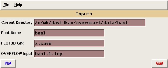
Figure 2. The main panel.

"Current Directory" is the name of the directory containing the run history files. The "Root Name" is the prefix of these history files. For example, if "Root Name"="basl", then OVERSMART will search for the following files: basl.resid, basl.turb, and basl.fomoco. "PLOT3D Grid" is the name of the grid file in PLOT3D format. For OVERFLOW runs, grid files are either grid.in or x.save. "OVERFLOW Input" is the flow solver input parameters file.

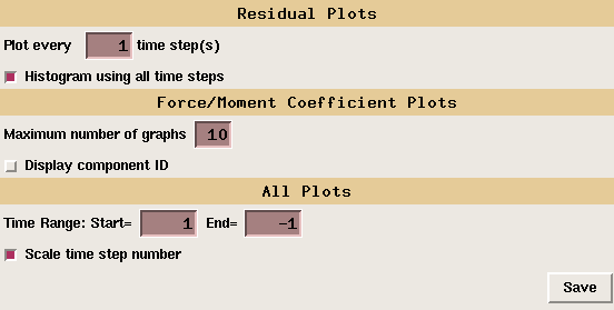
Figure 3. The preferences panel.

By default, OVERSMART plots every time step in the residual plot. User can override this default by specifing the "NSKIP" value in "Plot every NSKIP time step". This is very useful to take a quick look of the residual history files when there are thousands of time steps in these files. The Histogram plots are generated based on every time step in the residual history file. However, users may use those residuals from the every "NSKIP" time step by unselecting the option "Histogram using all time steps".

Two attributes of the Force/Moment coefficient plots can be specified. The first attribute is the maximum number of graphs that can be displayed. The second attribute specifies whether to display the components by its name or by its ID in the legend.

For all plots, users can specify the range of time steps to be displayed on the graph by specifying the starting and the ending time steps. If the time step numbers are large (e.g., greater than 10,000), then the tick labels on the time axis can be cluttered. To reduce the cluttering of the tick labels, OVERSMART will scale the time step numbers (default). To disable this feature, users can unselect the "Scale time step number" check button.

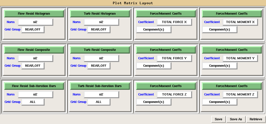
Figure 4. The command panel.

OVERSMART displays a matrix of plots for the executive summary page. For each sub-plot in the summary page, users can easily change the type of graph and the associate data variable to plot. Users can also save and retrieve previously saved summary page templates.

Limitations - The graphs displayed in the GUI viewing window normally do not have the same quality as those generated in the batch mode. For report quality plots, batch mode is recommended. The GUI mode in this version is a preliminary version and there may be some bugs/errors. Please report all bugs/erros and suggestions for improvement.

Future Work

Dynamic monitoring
Comparison plots between different runs
Auto convergence analysis and detection
Multi-threaded mode

Known Issues

When Gnuplot is specified, the plot page size is small. Hence, some legends and labels will overlap. To avoid this problem, plot only a small number of plots in the summary page (e.g., 2x2). The GUI mode of OVERSMART is still under further testing.

Acknowledgements

The replacement of matplotlib (the default plotting package in the previous version of OVERSMART) with xmGrace was mostly completed by Nick Kowlackzy as part of his internship during Summer 2013.

Publications

Kao, D. L., Chan, W. M., "OVERSMART - A Solution Monitoring and Reporting Tool for the OVERFLOW Flow Solver," AIAA Paper 2009-3998, 19th AIAA Computational Fluid Dynamics Conference, San Antonio, Texas, June, 2009.

Appendix A: Default commands (data sets with sub-iterations)

	Resid SL2
	Grid Near, Off
	Histogram 
	Plot Row 1 Column 1

	Turb SL2  
	Grid Near, Off
	Histogram 
	Plot Row 1 Column 2

	Fomoco TOTAL FORCE X
	Component All
	Plot Row 1 Column 3

	Fomoco TOTAL MOMENT X
	Component All
	Plot Row 1 Column 4

	Resid SL2  
	Grid Near, Off
	Composites
	Plot Row 2 Column 1

	Turb SL2  
	Grid Near, Off
	Composites
	Plot Row 2 Column 2

	Fomoco TOTAL FORCE Y
	Component All
	Plot Row 2 Column 3

	Fomoco TOTAL MOMENT Y
	Component All
	Plot Row 2 Column 4

	Resid SL2
	Grid All 
	SubIterBar 
	Plot Row 3 Column 1

	Turb SL2 
	Grid All 
	SubIterBar 
	Plot Row 3 Column 2

	Fomoco TOTAL FORCE Z
	Component All
	Plot Row 3 Column 3

	Fomoco TOTAL MOMENT Z
	Component All
	Plot Row 3 Column 4

Last modified: September 10, 2025